Orbit and phase-space position objects in more detail
Introduction
The astropy.units subpackage is excellent for working with numbers and
associated units, however, dynamical quantities often contain many
quantities with mixed units. An example is a position in phase-space, which
may contain some quantities with length units and some quantities with
velocity units. The PhaseSpacePosition and
Orbit subclasses are designed to work with these structures –
click these shortcuts to jump to a section below:
Some imports needed for the code below:
>>> import astropy.units as u
>>> import numpy as np
>>> import gala.potential as gp
>>> import gala.dynamics as gd
>>> from gala.units import galactic
>>> np.random.seed(42)
Phase-space positions
It is often useful to represent full phase-space positions quantities jointly.
For example, if you need to transform the velocities to a new coordinate
representation or frame, the positions often enter into the transformations.
The PhaseSpacePosition subclasses provide an interface for
handling these numbers. At present, only the
CartesianPhaseSpacePosition is fully implemented.
To create a CartesianPhaseSpacePosition object, pass in a
cartesian position and velocity to the initializer:
>>> gd.CartesianPhaseSpacePosition(pos=[4.,8.,15.]*u.kpc,
...                                vel=[-150.,50.,15.]*u.km/u.s)
<CartesianPhaseSpacePosition N=3, shape=(1,)>
Of course, this works with arrays of positions and velocities as well:
>>> x = np.random.uniform(-10,10,size=(3,128))
>>> v = np.random.uniform(-200,200,size=(3,128))
>>> gd.CartesianPhaseSpacePosition(pos=x*u.kpc,
...                                vel=v*u.km/u.s)
<CartesianPhaseSpacePosition N=3, shape=(128,)>
This works for arbitrary numbers of dimensions, e.g., we define a position:
>>> w = gd.CartesianPhaseSpacePosition(pos=[4.,8.]*u.kpc,
...                                    vel=[-150,45.]*u.km/u.s)
>>> w
<CartesianPhaseSpacePosition N=2, shape=(1,)>
We can check the dimensionality using the ndim
attribute:
>>> w.ndim
2
For objects with ndim=3, we can also easily transform the full
phase-space vector to new representations or coordinate frames. These
transformations use the astropy.coordinates framework and the
velocity transforms from gala.coordinates.
>>> from astropy.coordinates import CylindricalRepresentation
>>> x = np.random.uniform(-10,10,size=(3,128))
>>> v = np.random.uniform(-200,200,size=(3,128))
>>> w = gd.CartesianPhaseSpacePosition(pos=x*u.kpc,
...                                    vel=v*u.km/u.s)
>>> cyl_pos, cyl_vel = w.represent_as(CylindricalRepresentation)
The represent_as method returns two
objects that contain the position in the new representation, and the velocity
in the new representation. The position is returned as a
BaseRepresentation subclass. The velocity is
presently returned as a single Quantity object with
the velocity components represented in velocity units (not in angular velocity
units!) but this will change in the future when velocity support is added
to Astropy:
>>> cyl_pos
<CylindricalRepresentation (rho, phi, z) in (kpc, rad, kpc)
    [(2.64929392, 1.5595981, 5.27411405),
...etc.
>>> cyl_vel
<Quantity [[-185.61668456, 160.10813427, -75.14559842, 138.36905651,
             -60.93410629,  95.60242757,  41.89615149, 128.34632582,
...etc.
There is also support for transforming the cartesian positions and velocities
(assumed to be in a Galactocentric frame) to any of
the other coordinate frames. The transformation returns two objects: an
initialized coordinate frame for the position, and a tuple of
Quantity objects for the velocity. Here, velocities
are represented in angular velocities for the velocities conjugate to angle
variables. For example, in the below transformation to
Galactic coordinates, the returned velocity
object is a tuple with proper motions and radial velocity,
\((\mu_l, \mu_b, v_r)\):
>>> from astropy.coordinates import Galactic
>>> gal_c, gal_v = w.to_frame(Galactic)
>>> gal_c
<Galactic Coordinate: (l, b, distance) in (deg, deg, kpc)
    [(17.67673481, 31.15412806, 10.19473889),
...etc.
>>> gal_v[0].unit, gal_v[1].unit, gal_v[2].unit
(Unit("mas / yr"), Unit("mas / yr"), Unit("km / s"))
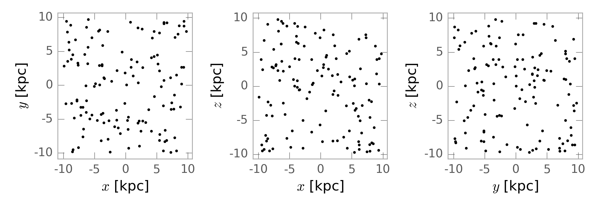
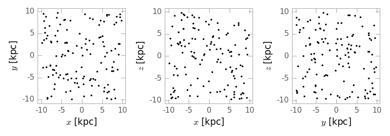
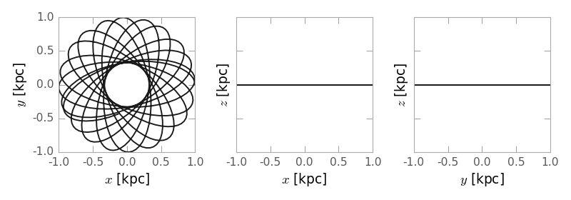
We can easily plot projections of the positions using the
plot method:
>>> fig = w.plot()
(Source code, png, hires.png, pdf)
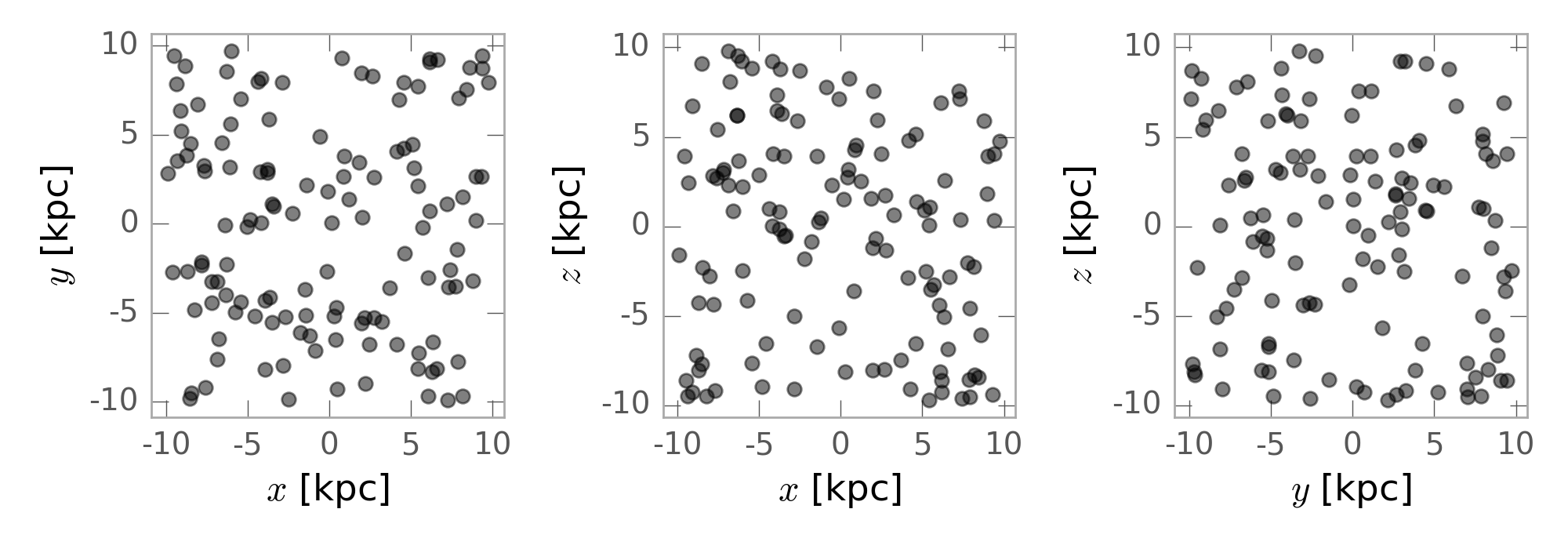
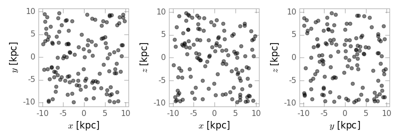
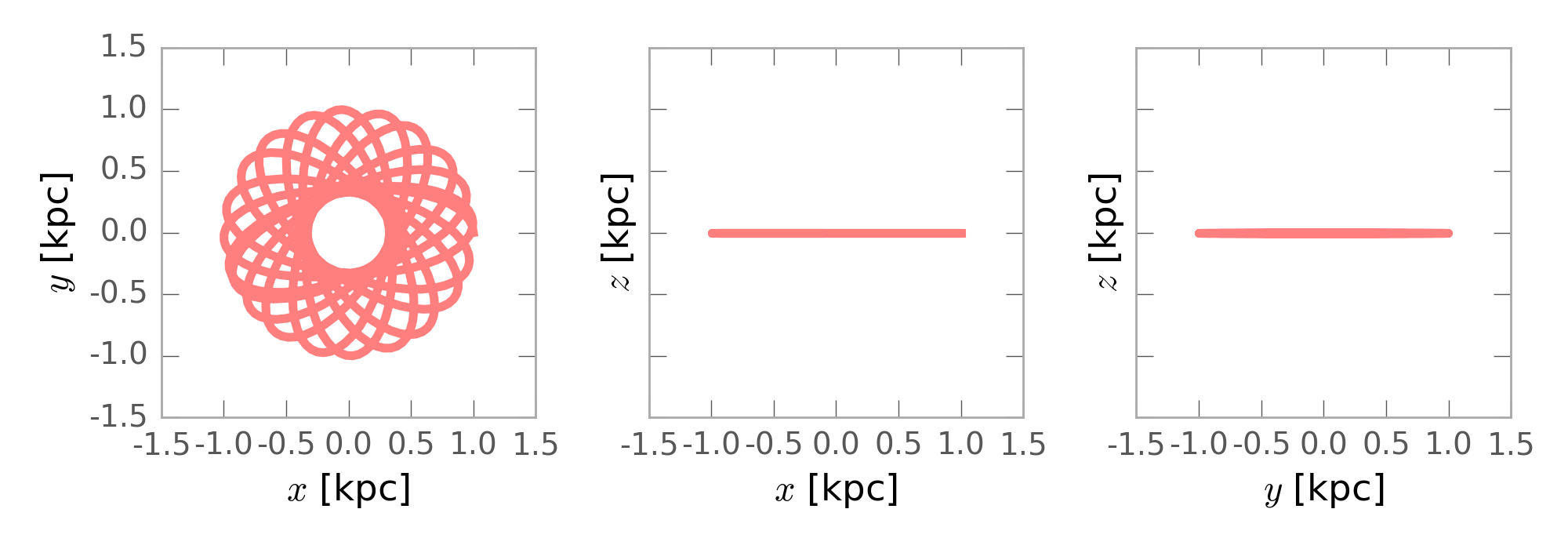
This is a thin wrapper around the three_panel
function and any keyword arguments are passed through to that function:
>>> fig = w.plot(marker='o', s=40, alpha=0.5)
(Source code, png, hires.png, pdf)
Phase-space position API
Classes
CartesianPhaseSpacePosition(pos, vel) |
Represents phase-space positions in Cartesian coordinates, e.g., positions and conjugate momenta (velocities). |
Class Inheritance Diagram
Orbits
The Orbit subclasses all inherit the functionality described
above from PhaseSpacePosition, but similarly, at present only the
CartesianOrbit is fully implemented. There are some differences
between the methods and some functionality that is particular to the orbit classes.
A CartesianOrbit is initialized much like the
CartesianPhaseSpacePosition. Whereas an input position with
shape ``(2,128)` to a CartesianPhaseSpacePosition represents
128, 2D positions, for an orbit it would represent a single orbit’s positions
at 128 timesteps:
>>> t = np.linspace(0,10,128)
>>> pos,vel = np.zeros((2,128)),np.zeros((2,128))
>>> pos[0] = np.cos(t)
>>> pos[1] = np.sin(t)
>>> vel[0] = -np.sin(t)
>>> vel[1] = np.cos(t)
>>> orbit = gd.CartesianOrbit(pos=pos*u.kpc, vel=vel*u.km/u.s)
>>> orbit
<CartesianOrbit N=2, shape=(128,)>
To create a single object that contains multiple orbits, the input position object
should have 3 axes. The last axis (axis=2) contains each orbit. So, an input
position with shape (2,128,16) would represent 16, 2D orbits with 128 timesteps:
>>> t = np.linspace(0,10,128)
>>> pos,vel = np.zeros((2,128,16)),np.zeros((2,128,16))
>>> Omega = np.random.uniform(size=16)
>>> pos[0] = np.cos(Omega[np.newaxis]*t[:,np.newaxis])
>>> pos[1] = np.sin(Omega[np.newaxis]*t[:,np.newaxis])
>>> vel[0] = -np.sin(Omega[np.newaxis]*t[:,np.newaxis])
>>> vel[1] = np.cos(Omega[np.newaxis]*t[:,np.newaxis])
>>> orbit = gd.CartesianOrbit(pos=pos*u.kpc, vel=vel*u.km/u.s)
>>> orbit
<CartesianOrbit N=2, shape=(128, 16)>
To make full use of the orbit functionality, you must also pass in an array with
the time values and an instance of a PotentialBase subclass that
represents the potential that the orbit was integrated in:
>>> pot = gp.PlummerPotential(m=1E10, b=1., units=galactic)
>>> orbit = gd.CartesianOrbit(pos=pos*u.kpc, vel=vel*u.km/u.s,
...                           t=t*u.Myr, potential=pot)
(note, in this case pos and vel were not generated from integrating
an orbit in the potential pot!) Orbit objects
are returned by the integrate_orbit method
of potential objects that already have the time and potential set:
>>> pot = gp.PlummerPotential(m=1E10, b=1., units=galactic)
>>> w0 = gd.CartesianPhaseSpacePosition(pos=[10.,0,0]*u.kpc,
...                                     vel=[0.,75,0]*u.km/u.s)
>>> orbit = pot.integrate_orbit(w0, dt=1., n_steps=500)
>>> orbit
<CartesianOrbit N=3, shape=(501,)>
>>> orbit.t
<Quantity [   0.,   1.,   2.,   3.,   4.,   5.,   6.,   7.,   8.,   9.,
             10.,  11.,  12.,  13.,  14.,  15.,  16.,  17.,  18.,  19.,
...etc.
>>> orbit.potential
<PlummerPotential: m=1.00e+10, b=1.00 (kpc,Myr,solMass,rad)>
From an Orbit object, we can quickly compute quantities like the angular momentum, and estimates for the pericenter, apocenter, eccentricity of the orbit. Estimates for the latter few get better with smaller timesteps:
>>> orbit = pot.integrate_orbit(w0, dt=0.1, n_steps=100000)
>>> np.mean(orbit.angular_momentum(), axis=1)
<Quantity [ 0.        , 0.        , 0.76703412] kpc2 / Myr>
>>> orbit.eccentricity()
<Quantity 0.3191563009914265>
>>> orbit.pericenter()
<Quantity 10.00000005952518 kpc>
>>> orbit.apocenter()
<Quantity 19.375317870528118 kpc>
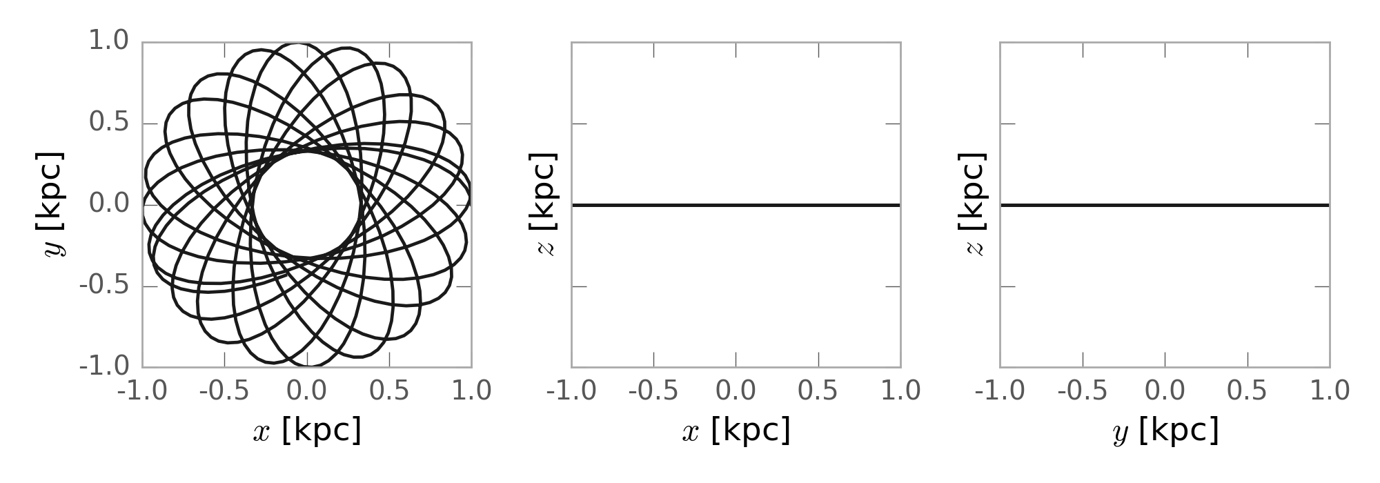
Just like above, we can quickly visualize an orbit using the
plot method:
>>> fig = orbit.plot()
(Source code, png, hires.png, pdf)
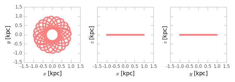
This is a thin wrapper around the plot_orbits
function and any keyword arguments are passed through to that function:
>>> fig = orbit.plot(linewidth=4., alpha=0.5, color='r')
>>> fig.axes[0].set_xlim(-1.5,1.5)
>>> fig.axes[0].set_ylim(-1.5,1.5)
(Source code, png, hires.png, pdf)
