Integration (gala.integrate)
Introduction
Scipy provides numerical ODE integration functions but they aren’t very user friendly or object oriented. This subpackage implements the Leapfrog integration scheme (not available in Scipy) and provides wrappers to higher order integration schemes such as a 5th order Runge-Kutta and the Dormand-Prince 85(3) method.
For code blocks below and any pages linked below, I assume the following imports have already been executed:
>>> import astropy.units as u
>>> import numpy as np
>>> import gala.integrate as gi
>>> from gala.units import galactic
Getting Started
All of the integrator classes have the same basic call structure. To create an
integrator object, you pass in a function that evaluates derivatives of, for
example, phase-space coordinates, then you call the
run method while specifying timestep information.
The integration function must accept, at minimum, two arguments: the current
time, t, and the current position in phase-space, w. The time is a
single floating-point number and the position will have shape (ndim,
norbits) where ndim is the full dimensionality of the phase-space (e.g., 6
for a 3D coordinate system) and norbits is the number of orbits. These
inputs will not have units associated with them (e.g., they are not
astropy.units.Quantity objects). An example of such a function (that
represents a simple harmonic oscillator) is:
>>> def F(t, w):
...     x,x_dot = w
...     return np.array([x_dot, -x])
Even though time does not explicitly enter into the equation, the function must
still accept a time argument. We will now create an instance of
LeapfrogIntegrator to integrate an orbit:
>>> integrator = gi.LeapfrogIntegrator(F)
To actually run the integrator, we need to specify a set of initial conditions. The simplest way to do this is to specify an array:
>>> w0 = np.array([1.,0.])
However this then causes the integrator to work without units. The orbit object returned by the integrator will then also have no associated units. For example, to integrate from these initial conditions with a time step of 0.5 for 100 steps:
>>> orbit = integrator.run(w0, dt=0.5, n_steps=100)
>>> orbit.t.unit
Unit(dimensionless)
>>> orbit.pos.xyz.unit
Unit(dimensionless)
We can instead specify the unit system that the function (F) expects, and
then pass in a PhaseSpacePosition object with arbitrary units
in as initial conditions:
>>> import gala.dynamics as gd
>>> from gala.units import UnitSystem
>>> usys = UnitSystem(u.m, u.s, u.kg, u.radian)
>>> integrator = gi.LeapfrogIntegrator(F, func_units=usys)
>>> w0 = gd.PhaseSpacePosition(pos=[100.]*u.cm, vel=[0]*u.cm/u.yr)
>>> orbit = integrator.run(w0, dt=0.5, n_steps=100)
>>> orbit.t.unit
Unit("s")
Now the orbit object will have quantities in the specified unit system.
Example: Forced pendulum
Here we demonstrate how to use the Dormand-Prince integrator to compute the
orbit of a forced pendulum. We will use the variable q as the angle of the
pendulum with respect to the vertical and p as the conjugate momentum. Our
Hamiltonian is
so that
Our derivative function is then:
>>> def F(t, w, A, omega_D):
...     q,p = w
...     q_dot = p
...     p_dot = -np.sin(q) + A*omega_D*np.cos(omega_D*t)
...     return np.array([q_dot, p_dot])
This function has two arguments – \(A\) (A), the amplitude of the
forcing, and \(\omega_D\) (omega_D), the driving frequency. We define an
integrator object by specifying this function, along with values for the
function arguments:
>>> integrator = gi.DOPRI853Integrator(F, func_args=(0.07, 0.75))
To integrate an orbit, we use the run method. We
have to specify the initial conditions along with information about how long to
integrate and with what stepsize. There are several options for how to specify
the time step information. We could pre-generate an array of times and pass that
in, or pass in an initial time, end time, and timestep. Or, we could simply pass
in the number of steps to run for and a timestep. For this example, we will use
the last option. See the API below under “Other Parameters” for more
information.:
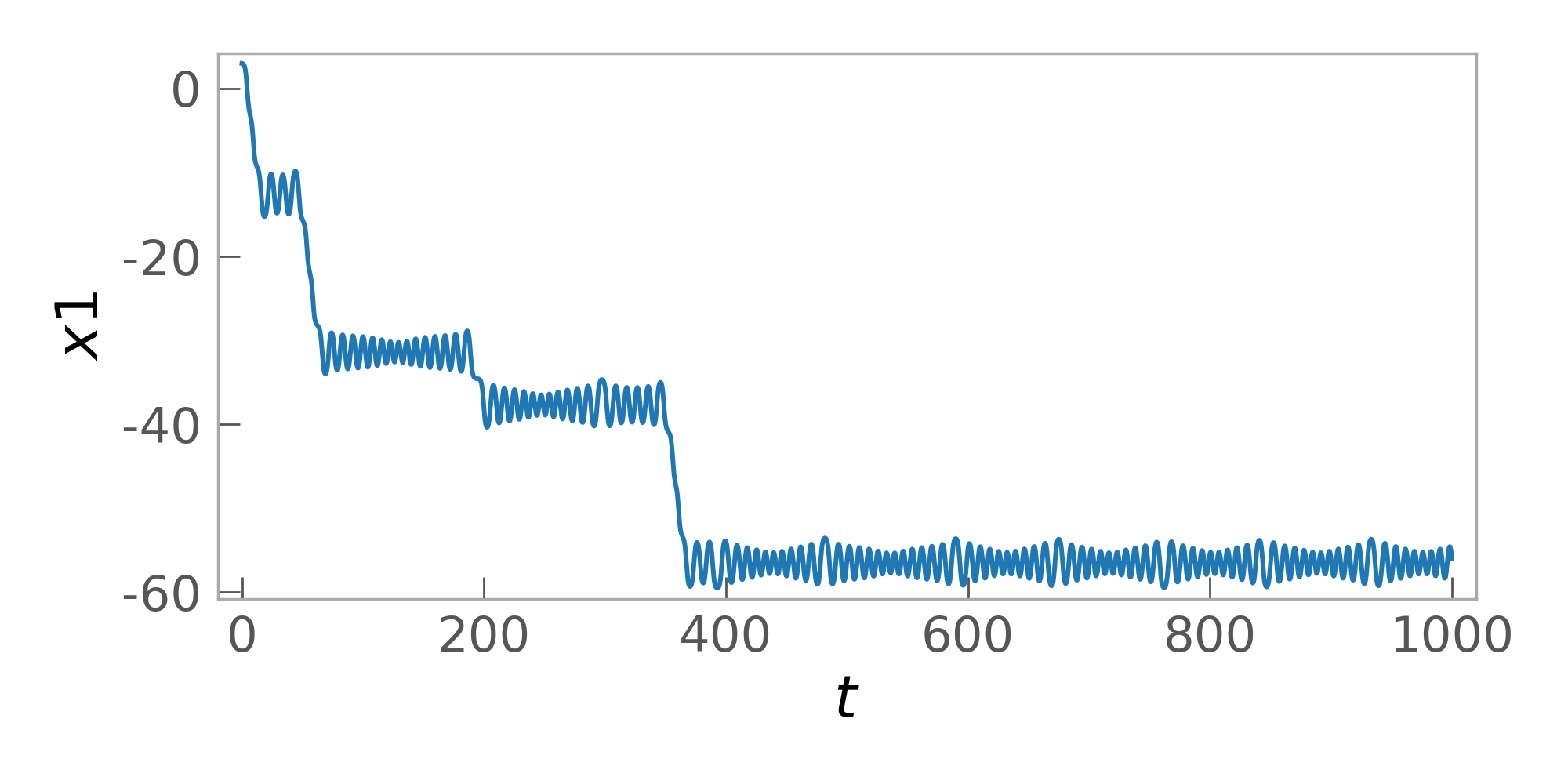
>>> orbit = integrator.run([3.,0.], dt=0.1, n_steps=10000)
We can plot the integrated (chaotic) orbit:
>>> fig = orbit.plot(subplots_kwargs=dict(figsize=(8,4)))
(Source code, png)
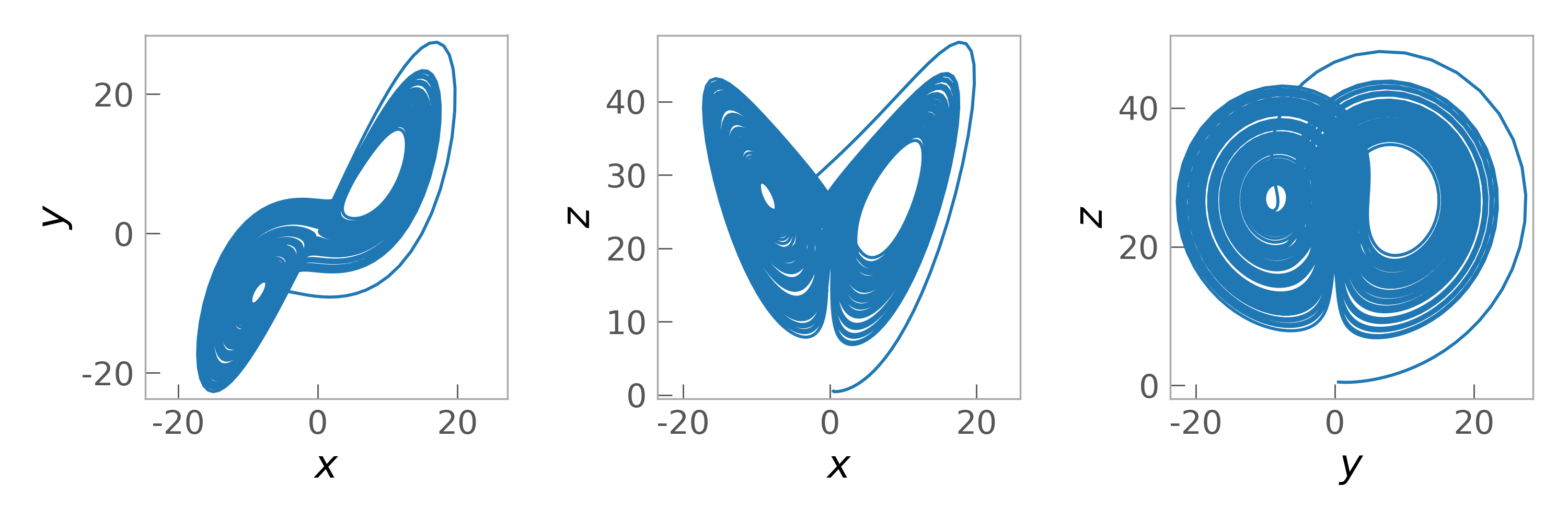
Example: Lorenz equations
Here’s another example of integrating the Lorenz equations, a 3D nonlinear system:
>>> def F(t,w,sigma,rho,beta):
...     x,y,z,px,py,pz = w
...     return np.array([sigma*(y-x), x*(rho-z)-y, x*y-beta*z, 0., 0., 0.]).reshape(w.shape)
>>> sigma, rho, beta = 10., 28., 8/3.
>>> integrator = gi.DOPRI853Integrator(F, func_args=(sigma, rho, beta))
>>> orbit = integrator.run([0.5,0.5,0.5,0,0,0], dt=1E-2, n_steps=1E4)
>>> fig = orbit.plot()
(Source code, png)
API
gala.integrate Package
Functions
parse_time_specification(units[, dt, …]) |
Return an array of times given a few combinations of kwargs that are accepted – see below. |
Classes
DOPRI853Integrator(func[, func_args, …]) |
This provides a wrapper around Scipy’s implementation of the Dormand-Prince 85(3) integration scheme. |
LeapfrogIntegrator(func[, func_args, …]) |
A symplectic, Leapfrog integrator. |
RK5Integrator(func[, func_args, func_units, …]) |
Initialize a 5th order Runge-Kutta integrator given a function for computing derivatives with respect to the independent variables. |