Dynamics (gala.dynamics)
For code blocks below and any pages linked below, we’ll assume the following imports have already been executed:
>>> import astropy.units as u
>>> import numpy as np
>>> import gala.potential as gp
>>> import gala.dynamics as gd
>>> from gala.units import galactic
Introduction
This subpackage contains functions and classes useful for gravitational dynamics. There are utilities for transforming orbits in phase-space to action-angle coordinates, tools for visualizing and computing dynamical quantities from orbits, tools to generate mock stellar streams, and tools useful for nonlinear dynamics such as Lyapunov exponent estimation.
The fundamental objects used by many of the functions and utilities in this and
other subpackages are the PhaseSpacePosition and Orbit classes.
Getting started: Working with orbits
As a demonstration of how to use these objects, we’ll start by integrating an
orbit using the gala.potential and gala.integrate subpackages:
>>> pot = gp.MiyamotoNagaiPotential(m=2.5E11*u.Msun, a=6.5*u.kpc,
...                                 b=0.26*u.kpc, units=galactic)
>>> w0 = gd.PhaseSpacePosition(pos=[11., 0., 0.2]*u.kpc,
...                            vel=[0., 200, 100]*u.km/u.s)
>>> orbit = gp.Hamiltonian(pot).integrate_orbit(w0, dt=1., n_steps=1000)
This numerically integrates an orbit from the specified initial conditions,
w0, and returns an Orbit object. By default, the position and velocity are
assumed to be Cartesian coordinates but other coordinate systems are supported
(see the Orbit and phase-space position objects in more detail and N-dimensional representation classes pages for more
information).
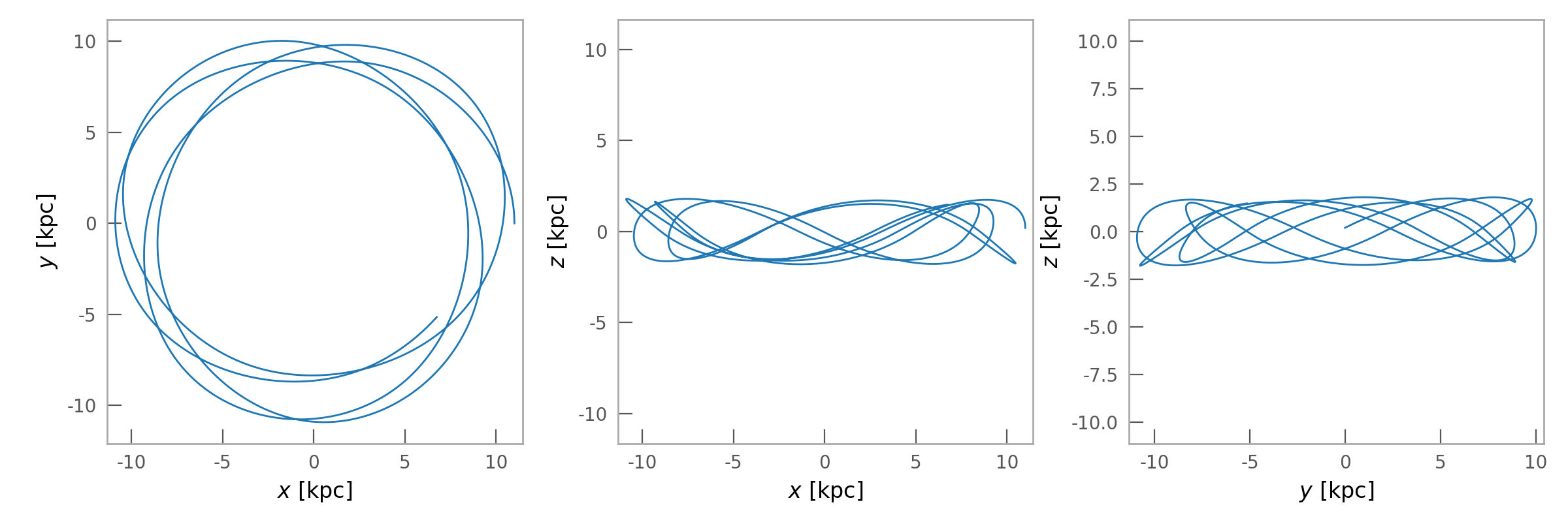
The Orbit object that is returned contains many useful methods, and can be
passed to many of the analysis functions implemented in Gala. For example, we
can easily visualize the orbit by plotting the time series in all Cartesian
projections using the plot() method:
>>> fig = orbit.plot()
(Source code, png)
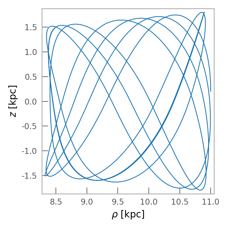
Or, we can visualize the orbit in just one projection of some transformed coordinate representation, for example, cylindrical radius \(\rho\) and \(z\):
>>> fig = orbit.represent_as('cylindrical').plot(['rho', 'z'])
(Source code, png)

From the Orbit object, we can also easily compute dynamical quantities such as
the energy or angular momentum (we take the 0th element because these functions
return the quantities computed at every timestep):
>>> E = orbit.energy()
>>> E[0]
<Quantity −0.060740198 kpc2 / Myr2>
Let’s see how well the integrator conserves energy and the z component of
angular momentum:
>>> Lz = orbit.angular_momentum()[2]
>>> np.std(E), np.std(Lz)
(<Quantity 4.654233175716351e-06 kpc2 / Myr2>,
 <Quantity 9.675900603446092e-16 kpc2 / Myr>)
We can access the position and velocity components of the orbit separately using
attributes that map to the underlying BaseRepresentation
and BaseDifferential subclass instances that store the
position and velocity data. The attribute names depend on the representation.
For example, for a Cartesian representation, the position components are ['x',
'y', 'z'] and the velocity components are ['v_x', 'v_y', 'v_z']. With a
Orbit or PhaseSpacePosition instance, you can check the valid compnent names using the
attributes .pos_components and .vel_components:
>>> orbit.pos_components.keys()
odict_keys(['x', 'y', 'z'])
>>> orbit.vel_components.keys()
odict_keys(['v_x', 'v_y', 'v_z'])
Meaning, we can access these components by doing, e.g.:
>>> orbit.v_x
<Quantity [ 0.        ,-0.00567589,-0.01129934,...,  0.18751756,
            0.18286687, 0.17812762] kpc / Myr>
For a Cylindrical representation, these are instead:
>>> cyl_orbit = orbit.represent_as('cylindrical')
>>> cyl_orbit.pos_components.keys()
odict_keys(['rho', 'phi', 'z'])
>>> cyl_orbit.vel_components.keys()
odict_keys(['v_rho', 'pm_phi', 'v_z'])
>>> cyl_orbit.v_rho
<Quantity [ 0.        ,-0.00187214,-0.00369183,...,  0.01699321,
            0.01930216, 0.02159477] kpc / Myr>
Continue to the Orbit and phase-space position objects in more detail page for more information.
Using gala.dynamics
More details are provided in the linked pages below:
gala.dynamics Package
Functions
|
Returns a list of the index of elements of n which do not have adequate toy angle coverage. |
|
Combine the specified |
|
DEPRECATED! |
|
Estimate the timestep and number of steps to integrate an orbit for given its initial conditions and a potential object. |
|
This function has been deprecated! |
|
Compute the maximum Lyapunov exponent using a C-implemented estimator that uses the DOPRI853 integrator. |
|
Find approximate actions and angles for samples of a phase-space orbit. |
|
Fit the toy harmonic oscillator potential to the sum of the energy residuals relative to the mean energy by minimizing the function |
|
Fit the toy Isochrone potential to the sum of the energy residuals relative to the mean energy by minimizing the function |
|
Fit a best fitting toy potential to the orbit provided. |
|
Generate integer vectors, \(\boldsymbol{n}\), with \(|\boldsymbol{n}| < N_{\rm max}\). |
|
Transform the input cartesian position and velocity to action-angle coordinates for the Harmonic Oscillator potential. |
|
Transform the input cartesian position and velocity to action-angle coordinates in the Isochrone potential. |
|
Compute the maximum Lyapunov exponent of an orbit by integrating many nearby orbits ( |
|
DEPRECATED! |
|
|
|
Estimate the period of the input time series by measuring the average peak-to-peak time. |
|
Given N-dimensional quantity, |
|
This function has been deprecated! |
|
Generate and return a surface of section from the given orbit. |
Classes
|
A base class for representing distribution functions for generating stellar streams. |
|
Deprecated. |
|
Perform orbit integration using direct N-body forces between particles, optionally in an external background potential. |
A class for representing the Fardal+2015 distribution function for generating stellar streams based on Fardal et al.2015. |
|
|
A class for representing the Lagrange Cloud Stripping distribution function for generating stellar streams. |
|
Represents phase-space positions, i.e. |
|
Generate a mock stellar stream in the specified external potential. |
|
Differentials in of points in ND cartesian coordinates. |
|
Representation of points in ND cartesian coordinates. |
|
Represents an orbit: positions and velocities (conjugate momenta) as a function of time. |
|
Represents phase-space positions, i.e. |
A class for representing the “streakline” distribution function for generating stellar streams based on Kuepper et al.2012. |