Compute an SCF representation of an arbitrary density distribution
Basis function expansions are a useful tool for computing gravitational potentials and forces from an arbitrary density function that may not have an analytic solution to Poisson’s equation. They are also useful for generating smoothed or compressed representations of gravitational potentials from discrete particle distributions. For astronomical density distributions, a useful expansion technique is the Self-Consistent Field (SCF) method, as initially developed by Hernquist & Ostriker (1992). In this method, using the notation of Lowing et al. 2011, the density and potential functions are expressed as:
where \(Y_{lm}(\theta)\) are the usual spherical harmonics, \(\rho_{nlm}(r)\) and \(\Phi_{nlm}(r)\) are bi-orthogonal radial basis functions, and \(S_{nlm}\) and \(T_{nlm}\) are expansion coefficients, which need to be computed from a given density function. In this notebook, we’ll estimate low-order expansion coefficients for an analytic density distribution (written as a Python function).
[1]:
# Some imports we'll need later:

# Third-party
import astropy.units as u
import matplotlib.pyplot as plt
import numpy as np
%matplotlib inline

# Custom
import gala.coordinates as gc
import gala.dynamics as gd
import gala.integrate as gi
import gala.potential as gp
from gala.units import galactic
from gala.potential.scf import compute_coeffs, compute_coeffs_discrete
SCF representation of an analytic density distribution
Custom spherical density function
For this example, we’ll assume that we want a potential representation of the spherical density function:
Let’s start by writing a density function that takes a single set of Cartesian coordinates (x, y, z) and returns the (scalar) value of the density at that location:
[2]:
def density_func(x, y, z):
    r = np.sqrt(x**2 + y**2 + z**2)
    return 1 / (r**1.8 * (1 + r)**2.7)
Let’s visualize this density function. For comparison, let’s also over-plot the Hernquist density distribution. The SCF expansion uses the Hernquist density for radial basis functions, so the similarity of the density we want to represent and the Hernquist function gives us a sense of how many radial terms we will need in the expansion:
[3]:
hern = gp.HernquistPotential(m=1, c=1)
[4]:
x = np.logspace(-1, 1, 128)
plt.plot(x, density_func(x, 0, 0), marker='', label='custom density')

# need a 3D grid for the potentials in Gala
xyz = np.zeros((3, len(x)))
xyz[0] = x
plt.plot(x, hern.density(xyz), marker='', label='Hernquist')

plt.xscale('log')
plt.yscale('log')

plt.xlabel('$r$')
plt.ylabel(r'$\rho(r)$')

plt.legend(loc='best');
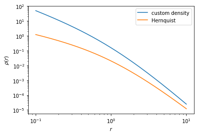
These functions are not too different, implying that we probably don’t need too many radial expansion terms in order to well represent the density/potential from this custom function. As an arbitrary number, let’s choose to compute radial terms up to and including \(n = 10\). In this case, because the density we want to represent is spherical, we don’t need any \(l, m\) terms, so we set lmax=0. We can also neglect the sin() terms of the expansion (\(T_{nlm}\)):
[5]:
(S, Serr), _ = compute_coeffs(density_func,
                              nmax=10, lmax=0,
                              M=1., r_s=1., S_only=True)
The above variable S will contain the expansion coefficients, and the variable Serr will contain an estimate of the error in this coefficient value. Let’s now construct an SCFPotential object with the coefficients we just computed:
[6]:
pot = gp.SCFPotential(m=1., r_s=1, Snlm=S)
Now let’s visualize the SCF estimated density with the true density:
[7]:
x = np.logspace(-1, 1, 128)
plt.plot(x, density_func(x, 0, 0), marker='', label='custom density')

# need a 3D grid for the potentials in Gala
xyz = np.zeros((3, len(x)))
xyz[0] = x
plt.plot(x, pot.density(xyz), marker='', label='SCF density')

plt.xscale('log')
plt.yscale('log')

plt.xlabel('$r$')
plt.ylabel(r'$\rho(r)$')

plt.legend(loc='best');
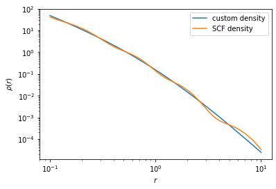
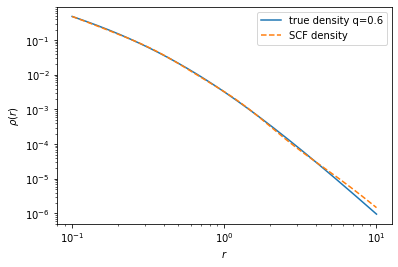
This does a pretty good job of capturing the radial fall-off of our custom density function, but you may want to iterate a bit to satisfy your own constraints. For example, you may want the density to be represented with a less than 1% deviation over some range of radii, or whatever.
As a second example, let’s now try a custom axisymmetric density distribution:
Custom axisymmetric density function
For this example, we’ll assume that we want a potential representation of the flattened Hernquist density function:
Let’s again start by writing a density function that takes a single set of Cartesian coordinates (x, y, z) and returns the (scalar) value of the density at that location:
[8]:
def density_func_flat(x, y, z, q):
    r = np.sqrt(x**2 + y**2 + (z / q)**2)
    return 1 / (r * (1 + r)**3) / (2*np.pi)
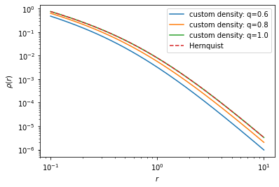
Let’s compute the density along a diagonal line for a few different flattenings and again compare to the non-flattened Hernquist profile:
[9]:
x = np.logspace(-1, 1, 128)
xyz = np.zeros((3, len(x)))
xyz[0] = x
xyz[2] = x

for q in np.arange(0.6, 1+1e-3, 0.2):
    plt.plot(x, density_func_flat(xyz[0], 0., xyz[2], q), marker='', label='custom density: q={0}'.format(q))

plt.plot(x, hern.density(xyz), marker='', ls='--', label='Hernquist')

plt.xscale('log')
plt.yscale('log')

plt.xlabel('$r$')
plt.ylabel(r'$\rho(r)$')

plt.legend(loc='best');
Because this is an axisymmetric density distribution, we need to also compute \(l\) terms in the expansion, so we set lmax=6, but we can skip the \(m\) terms using skip_m=True. Because this computes more coefficients, we might want to see the progress in real time - if you install the Python package tqdm and pass progress=True, it will also display a progress bar:
[10]:
q = 0.6
(S_flat, Serr_flat), _ = compute_coeffs(density_func_flat,
                                        nmax=4, lmax=6, args=(q, ),
                                        M=1., r_s=1., S_only=True,
                                        skip_m=True, progress=True)
100%|██████████| 35/35 [00:04<00:00, 7.42it/s]
[11]:
pot_flat = gp.SCFPotential(m=1., r_s=1, Snlm=S_flat)
[12]:
x = np.logspace(-1, 1, 128)
xyz = np.zeros((3, len(x)))
xyz[0] = x
xyz[2] = x

plt.plot(x, density_func_flat(xyz[0], xyz[1], xyz[2], q), marker='',
         label='true density q={0}'.format(q))

plt.plot(x, pot_flat.density(xyz), marker='', ls='--', label='SCF density')

plt.xscale('log')
plt.yscale('log')

plt.xlabel('$r$')
plt.ylabel(r'$\rho(r)$')

plt.legend(loc='best');
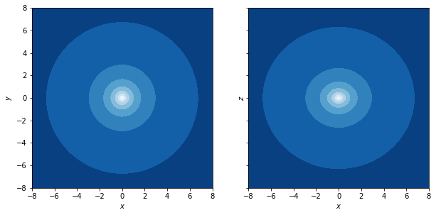
The SCF potential object acts like any other gala.potential object, meaning we can, e.g., plot density or potential contours:
[13]:
grid = np.linspace(-8, 8, 128)

fig, axes = plt.subplots(1, 2, figsize=(10, 5),
                         sharex=True, sharey=True)
_ = pot_flat.plot_contours((grid, grid, 0), ax=axes[0])
axes[0].set_xlabel('$x$')
axes[0].set_ylabel('$y$')

_ = pot_flat.plot_contours((grid, 0, grid), ax=axes[1])
axes[1].set_xlabel('$x$')
axes[1].set_ylabel('$z$')

for ax in axes:
    ax.set_aspect('equal')
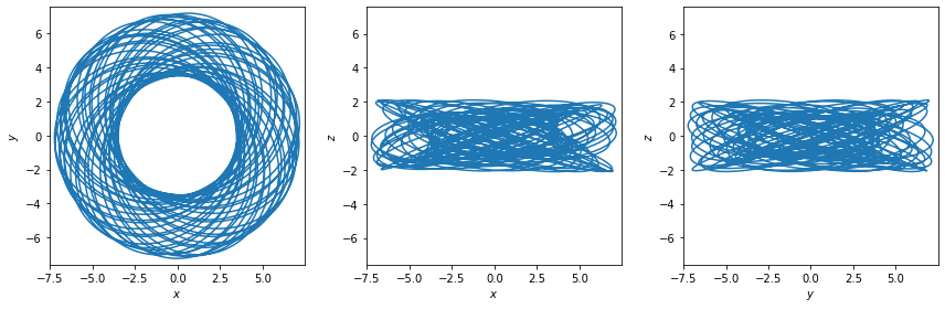
And numerically integrate orbits by passing in initial conditions and integration parameters:
[14]:
w0 = gd.PhaseSpacePosition(pos=[3.5, 0, 1],
                           vel=[0, 0.4, 0.05])
[15]:
orbit_flat = pot_flat.integrate_orbit(w0, dt=1., n_steps=5000)
_ = orbit_flat.plot()