Generating a mock stellar stream and converting to Heliocentric coordinates
We first need to import some relevant packages:
>>> import astropy.coordinates as coord
>>> import astropy.units as u
>>> import numpy as np
>>> import gala.coordinates as gc
>>> import gala.dynamics as gd
>>> import gala.potential as gp
>>> from gala.units import galactic
We will also set the default Astropy Galactocentric frame parameters to the values adopted in Astropy v4.0:
>>> _ = coord.galactocentric_frame_defaults.set('v4.0')
In the examples below, we will use the galactic
UnitSystem: as I define it, this is: \({\rm kpc}\),
\({\rm Myr}\), \({\rm M}_\odot\).
We first create a potential object to work with. For this example, we’ll use a two-component potential: a Miyamoto-Nagai disk with a spherical NFW potential to represent a dark matter halo.
>>> pot = gp.CCompositePotential()
>>> pot['disk'] = gp.MiyamotoNagaiPotential(m=6E10*u.Msun,
...                                         a=3.5*u.kpc, b=280*u.pc,
...                                         units=galactic)
>>> pot['halo'] = gp.NFWPotential(m=7E11, r_s=15*u.kpc, units=galactic)
We’ll use the Palomar 5 globular cluster and stream as a motivation for this example. For the position and velocity of the cluster, we’ll use \((\alpha, \delta) = (229, −0.124)~{\rm deg}\) [odenkirchen02], \(d = 22.9~{\rm kpc}\) [bovy16], \(v_r = -58.7~{\rm km}~{\rm s}^{-1}\) [bovy16], and \((\mu_{\alpha,*}, \mu_\delta) = (-2.296,-2.257)~{\rm mas}~{\rm yr}^{-1}\) [fritz15]:
>>> c = coord.ICRS(ra=229 * u.deg, dec=-0.124 * u.deg,
...                distance=22.9 * u.kpc,
...                pm_ra_cosdec=-2.296 * u.mas/u.yr,
...                pm_dec=-2.257 * u.mas/u.yr,
...                radial_velocity=-58.7 * u.km/u.s)
We’ll first convert this position and velocity to Galactocentric coordinates:
>>> c_gc = c.transform_to(coord.Galactocentric).cartesian
>>> c_gc
<CartesianRepresentation (x, y, z) in kpc
   (7.86390455, 0.22748727, 16.41622487)
(has differentials w.r.t.: 's')>
>>> pal5_w0 = gd.PhaseSpacePosition(c_gc)
We can now use the position and velocity of the cluster to generate a mock stellar stream with a progenitor that ends up at the present-day position of the cluster. We will generate a stream using the prescription defined in [fardal15], but including the self-gravity of the cluster mass itself. We will represent the cluster with a Plummer potential, with mass \(2.5 \times 10^4~{\rm M}_\odot\):
>>> pal5_mass = 2.5e4 * u.Msun
>>> pal5_pot = gp.PlummerPotential(m=pal5_mass, b=4*u.pc, units=galactic)
We now have to specify that we want to use the Fardal method for generating
stream particle initial conditions by creating a
FardalStreamDF instance:
>>> from gala.dynamics import mockstream as ms
>>> df = ms.FardalStreamDF()
Finally, we can generate the stream using the
MockStreamGenerator:
>>> gen_pal5 = ms.MockStreamGenerator(df, pot,
...                                   progenitor_potential=pal5_pot)
>>> pal5_stream, _ = gen_pal5.run(pal5_w0, pal5_mass,
...                               dt=-1 * u.Myr, n_steps=4000)
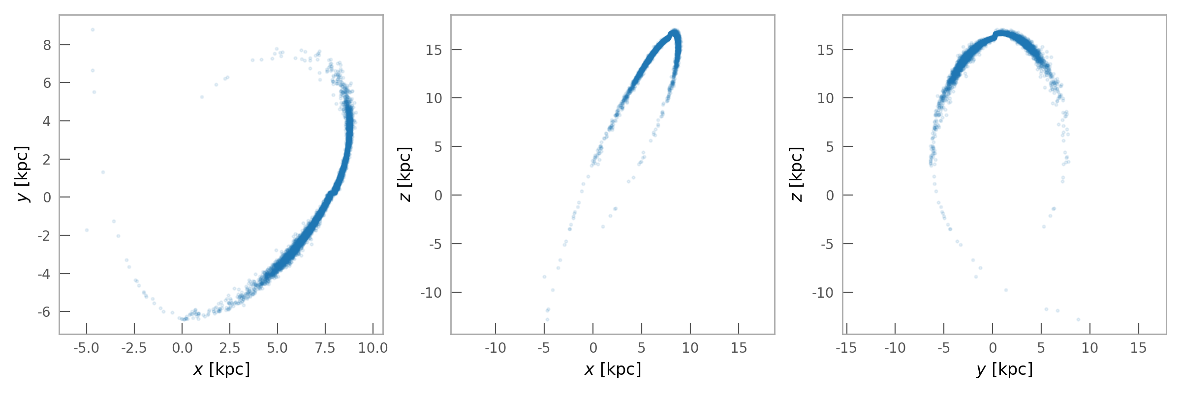
Here the negative timestep tells the stream generator to first integrate the orbit of the progenitor (the Pal 5 cluster itself) backwards in time, then generate the stream forwards from the past until present day:
>>> pal5_stream.plot(alpha=0.1)
(Source code, png)
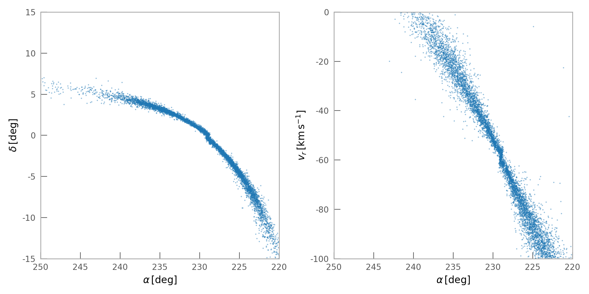
We now have the model stream particle positions and velocities in a Galactocentric coordinate frame. To convert these to observable, Heliocentric coordinates, we have to specify a desired coordinate frame. We’ll convert to the ICRS coordinate system and plot some of the Heliocentric kinematic quantities:
>>> stream_c = pal5_stream.to_coord_frame(coord.ICRS)
(Source code, png)