Defining a Milky Way potential model
[1]:
# Third-party dependencies
from astropy.io import ascii
import astropy.units as u
import numpy as np
import matplotlib.pyplot as plt
from scipy.optimize import leastsq

# Gala
from gala.mpl_style import mpl_style
plt.style.use(mpl_style)
import gala.dynamics as gd
import gala.integrate as gi
import gala.potential as gp
from gala.units import galactic
%matplotlib inline
Introduction
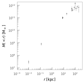
gala provides a simple and easy way to access and integrate orbits in an approximate mass model for the Milky Way. The parameters of the mass model are determined by least-squares fitting the enclosed mass profile of a pre-defined potential form to recent measurements compiled from the literature. These measurements are provided with the documentation of gala and are shown below. The radius units are kpc, and mass units are solar masses:
[2]:
tbl = ascii.read('data/MW_mass_enclosed.csv')
[3]:
tbl
[3]:
| r | Menc | Menc_err_neg | Menc_err_pos | ref |
|---|---|---|---|---|
| float64 | float64 | float64 | float64 | str27 |
| 0.01 | 30000000.0 | 10000000.0 | 10000000.0 | Feldmeier et al. (2014) |
| 0.12 | 800000000.0 | 200000000.0 | 200000000.0 | Launhardt et al. (2002) |
| 8.1 | 89502860861.52429 | 4994562473.797714 | 4858963492.608627 | Bovy et al. (2012) |
| 8.3 | 110417867208.19055 | 4475949382.696884 | 4387023236.020782 | McMillan (2011) |
| 8.4 | 102421035406.90356 | 16733918715.629944 | 15468328224.531876 | Koposov et al. (2010) |
| 19.0 | 208023299175.30438 | 44317988008.38101 | 34833267089.920685 | Kuepper et al. (2015) |
| 50.0 | 539884832748.48975 | 19995734543.31433 | 268490735257.4718 | Wilkinson & Evans (1999) |
| 50.0 | 529886965173.18726 | 9997867269.659302 | 38536752776.21277 | Sakamoto et al. (2003) |
| 50.0 | 399914690706.92847 | 109976539940.53711 | 72696676468.2511 | Smith et al. (2007) |
| 50.0 | 419910425325.7268 | 39991469076.968506 | 38172735113.64386 | Deason et al. (2012) |
| 60.0 | 399914690957.5188 | 69985070910.63354 | 64344945146.92987 | Xue et al. (2008) |
| 80.0 | 689852841359.0248 | 299936018002.3314 | 110361048549.1029 | Gnedin et al. (2010) |
| 100.0 | 1399701417307.7747 | 899808054059.3811 | 831336271726.1903 | Watkins et al. (2010) |
| 120.0 | 539884832260.29584 | 199957345314.72906 | 123854764645.32489 | Battaglia et al. (2005) |
| 150.0 | 750000000000.0 | 250000000000.0 | 250000000000.0 | Deason et al. (2012) |
| 200.0 | 679854974257.2006 | 409912558030.05396 | 313652012195.06256 | Bhattacherjee et al. (2014) |
Let’s now plot the above data and uncertainties:
[4]:
fig, ax = plt.subplots(1, 1, figsize=(4,4))

ax.errorbar(tbl['r'], tbl['Menc'], yerr=(tbl['Menc_err_neg'], tbl['Menc_err_pos']),
            marker='o', markersize=2, color='k', alpha=1., ecolor='#aaaaaa',
            capthick=0, linestyle='none', elinewidth=1.)

ax.set_xlim(1E-3, 10**2.6)
ax.set_ylim(7E6, 10**12.25)

ax.set_xlabel('$r$ [kpc]')
ax.set_ylabel('$M(<r)$ [M$_\odot$]')

ax.set_xscale('log')
ax.set_yscale('log')

fig.tight_layout()
We now need to assume some form for the potential. For simplicity and within reason, we’ll use a four component potential model consisting of a Hernquist (1990) bulge and nucleus, a Miyamoto-Nagai (1975) disk, and an NFW (1997) halo. We’ll fix the parameters of the disk and bulge to be
consistent with previous work (Bovy 2015 - please cite that paper if you use this potential model) and vary the scale mass and scale radius of the nucleus and halo, respectively. We’ll fit for these parameters in log-space, so we’ll first define a function that returns a gala.potential.CCompositePotential object given these four parameters:
[5]:
def get_potential(log_M_h, log_r_s, log_M_n, log_a):
    mw_potential = gp.CCompositePotential()
    mw_potential['bulge'] = gp.HernquistPotential(m=5E9, c=1., units=galactic)
    mw_potential['disk'] = gp.MiyamotoNagaiPotential(m=6.8E10*u.Msun, a=3*u.kpc, b=280*u.pc,
                                                     units=galactic)
    mw_potential['nucl'] = gp.HernquistPotential(m=np.exp(log_M_n), c=np.exp(log_a)*u.pc,
                                                 units=galactic)
    mw_potential['halo'] = gp.NFWPotential(m=np.exp(log_M_h), r_s=np.exp(log_r_s), units=galactic)

    return mw_potential
We now need to specify an initial guess for the parameters - let’s do that (by making them up), and then plot the initial guess potential over the data:
[6]:
# Initial guess for the parameters- units are:
#     [Msun, kpc, Msun, pc]
x0 = [np.log(6E11), np.log(20.), np.log(2E9), np.log(100.)]
init_potential = get_potential(*x0)
[7]:
xyz = np.zeros((3, 256))
xyz[0] = np.logspace(-3, 3, 256)

fig, ax = plt.subplots(1, 1, figsize=(4,4))

ax.errorbar(tbl['r'], tbl['Menc'], yerr=(tbl['Menc_err_neg'], tbl['Menc_err_pos']),
            marker='o', markersize=2, color='k', alpha=1., ecolor='#aaaaaa',
            capthick=0, linestyle='none', elinewidth=1.)

fit_menc = init_potential.mass_enclosed(xyz*u.kpc)
ax.loglog(xyz[0], fit_menc.value, marker='', color="#3182bd",
          linewidth=2, alpha=0.7)

ax.set_xlim(1E-3, 10**2.6)
ax.set_ylim(7E6, 10**12.25)

ax.set_xlabel('$r$ [kpc]')
ax.set_ylabel('$M(<r)$ [M$_\odot$]')

ax.set_xscale('log')
ax.set_yscale('log')

fig.tight_layout()
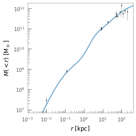
It looks pretty good already! But let’s now use least-squares fitting to optimize our nucleus and halo parameters. We first need to define an error function:
[8]:
def err_func(p, r, Menc, Menc_err):
    pot = get_potential(*p)
    xyz = np.zeros((3,len(r)))
    xyz[0] = r
    model_menc = pot.mass_enclosed(xyz).to(u.Msun).value
    return (model_menc - Menc) / Menc_err
Because the uncertainties are all approximately but not exactly symmetric, we’ll take the maximum of the upper and lower uncertainty values and assume that the uncertainties in the mass measurements are Gaussian (a bad but simple assumption):
[9]:
err = np.max([tbl['Menc_err_pos'], tbl['Menc_err_neg']], axis=0)
p_opt, ier = leastsq(err_func, x0=x0, args=(tbl['r'], tbl['Menc'], err))
assert ier in range(1,4+1), "least-squares fit failed!"
fit_potential = get_potential(*p_opt)
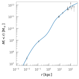
Now we have a best-fit potential! Let’s plot the enclosed mass of the fit potential over the data:
[10]:
xyz = np.zeros((3, 256))
xyz[0] = np.logspace(-3, 3, 256)

fig, ax = plt.subplots(1, 1, figsize=(4,4))

ax.errorbar(tbl['r'], tbl['Menc'], yerr=(tbl['Menc_err_neg'], tbl['Menc_err_pos']),
            marker='o', markersize=2, color='k', alpha=1., ecolor='#aaaaaa',
            capthick=0, linestyle='none', elinewidth=1.)

fit_menc = fit_potential.mass_enclosed(xyz*u.kpc)
ax.loglog(xyz[0], fit_menc.value, marker='', color="#3182bd",
          linewidth=2, alpha=0.7)

ax.set_xlim(1E-3, 10**2.6)
ax.set_ylim(7E6, 10**12.25)

ax.set_xlabel('$r$ [kpc]')
ax.set_ylabel('$M(<r)$ [M$_\odot$]')

ax.set_xscale('log')
ax.set_yscale('log')

fig.tight_layout()
This potential is already implemented in gala in gala.potential.special, and we can import it with:
[11]:
from gala.potential import MilkyWayPotential
[12]:
potential = MilkyWayPotential()
potential
[12]:
<CompositePotential disk,bulge,nucleus,halo>