Creating a multi-component potential

Potential objects can be combined into more complex composite potentials using the CompositePotential or CCompositePotential classes. These classes operate like a Python dictionary in that each component potential must be named, and the potentials can either be passed in to the initializer or added after the composite potential container is already created.

For composing any of the built-in potentials or any external potentials implemented in C, it is always faster to use CCompositePotential, where the composition is done at the C layer rather than in Python.

But with either class, interaction with the class is identical. Each component potential must be instantiated before adding it to the composite potential:

>>> import numpy as np
>>> import gala.potential as gp
>>> from gala.units import galactic
>>> disk = gp.MiyamotoNagaiPotential(m=1E11, a=6.5, b=0.27, units=galactic)
>>> bulge = gp.HernquistPotential(m=3E10, c=0.7, units=galactic)
>>> pot = gp.CCompositePotential(disk=disk, bulge=bulge)

is equivalent to:

>>> pot = gp.CCompositePotential()
>>> pot['disk'] = disk
>>> pot['bulge'] = bulge

In detail, the composite potential classes subclass OrderedDict, so in this sense there is a slight difference between the two examples above. By defining components after creating the instance, the order is preserved. In the above example, the disk potential would always be called first and the bulge would always be called second.

The resulting potential object has all of the same properties as individual potential objects:

>>> pot.value([1.,-1.,0.]) 
<Quantity [-0.12891172] kpc2 / Myr2>
>>> pot.acceleration([1.,-1.,0.]) 
<Quantity [[-0.02271507],
           [ 0.02271507],
           [-0.        ]] kpc / Myr2>
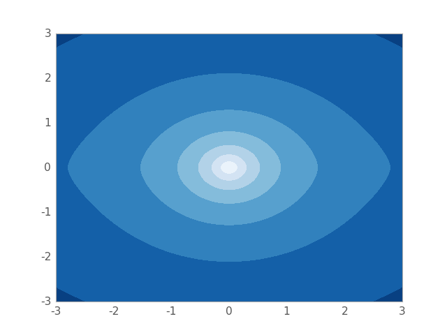
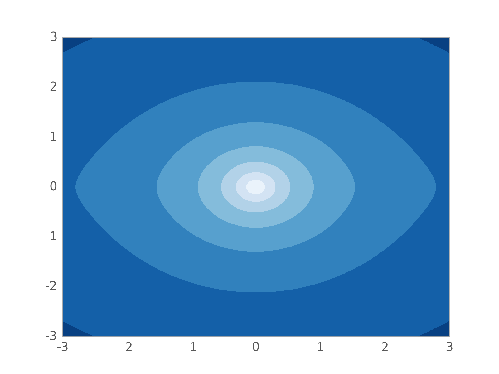
>>> grid = np.linspace(-3.,3.,100)
>>> fig = pot.plot_contours(grid=(grid,0,grid))

(Source code, png, hires.png, pdf)