Gravitational potentials (gala.potential)
Introduction
This subpackage provides a number of classes for working with parametric models
of gravitational potentials. There are base classes for creating custom
potential classes, but more useful are the built-in potentials. These are
commonly used potentials that have methods for computing, for example, the
potential value (energy), gradient, density, or mass profiles. These are
particularly useful in combination with the integrate and
dynamics subpackages.
For code blocks below and any pages linked below, I assume the following imports have already been excuted:
>>> import astropy.units as u
>>> import numpy as np
>>> import gala.potential as gp
>>> from gala.units import galactic, solarsystem, dimensionless
Getting started: built-in potential classes
The built-in potentials are all initialized by passing in keyword argument
parameter values as numeric values or Quantity objects.
To see what parameters are available for a given potential, check the
documentation for the individual classes below. You must also specify a
UnitSystem when initializing a potential. A unit system is a set
of non-reducible units that define the length, mass, time, and angle units. A
few common unit systems are built in to the package (e.g., solarsystem).
All of the built-in potential objects have defined methods that evaluate the value of the potential and the gradient/acceleration at a given position(s). For example, here we will create a potential object for a 2D point mass located at the origin with unit mass:
>>> ptmass = gp.KeplerPotential(m=1.*u.Msun, units=solarsystem)
>>> ptmass
<KeplerPotential: m=1.00 (AU,yr,solMass,rad)>
If you pass in parameters with different units, they will be converted to the specified unit system:
>>> gp.KeplerPotential(m=1047.6115*u.Mjup, units=solarsystem)
<KeplerPotential: m=1.00 (AU,yr,solMass,rad)>
If no units are specified for a parameter, it is assumed to already be
consistent with the UnitSystem passed in:
>>> gp.KeplerPotential(m=1., units=solarsystem)
<KeplerPotential: m=1.00 (AU,yr,solMass,rad)>
The potential classes work well with the astropy.units framework, but to
ignore units you can use the DimensionlessUnitSystem by
importing:
>>> from gala.units import dimensionless
>>> gp.KeplerPotential(m=1., units=dimensionless)
<KeplerPotential: m=1.00 (dimensionless)>
We can then evaluate the value of the potential at some position:
>>> ptmass.value([1.,-1.,0.]*u.au)
<Quantity [-27.92216622] AU2 / yr2>
These functions also accept plain ndarray-like objects where the
position is assumed to be in the unit system of the potential):
>>> ptmass.value([1.,-1.,0.])
<Quantity [-27.92216622] AU2 / yr2>
This also works for multiple positions by passing in a 2D position (but see Conventions for a description of the interpretation of different axes):
>>> pos = np.array([[1.,-1.,0],
...                 [2.,3.,0]]).T
>>> ptmass.value(pos*u.au)
<Quantity [-27.92216622,-10.95197465] AU2 / yr2>
We may also compute the gradient or acceleration:
>>> ptmass.gradient([1.,-1.,0]*u.au)
<Quantity [[ 13.96108311],
           [-13.96108311],
           [  0.        ]] AU / yr2>
>>> ptmass.acceleration([1.,-1.,0]*u.au)
<Quantity [[-13.96108311],
           [ 13.96108311],
           [ -0.        ]] AU / yr2>
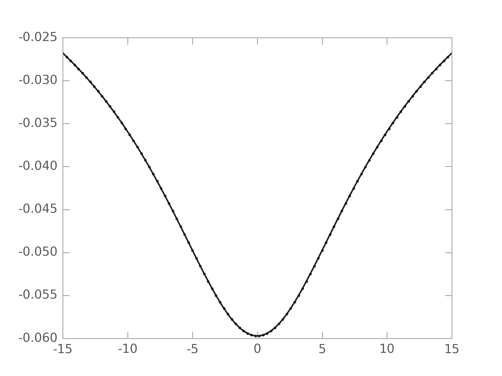
plot_contours supports plotting
either 1D slices or 2D contour plots of isopotentials. To plot a 1D slice
over the dimension of interest, pass in a grid of values for that dimension
and numerical values for the others. For example, to make a 1D plot of the
potential value as a function of \(x\) position at \(y=0, z=1\):
>>> p = gp.MiyamotoNagaiPotential(m=1E11, a=6.5, b=0.27, units=galactic)
>>> p.plot_contours(grid=(np.linspace(-15,15,100), 0., 1.))
(Source code, png, hires.png, pdf)

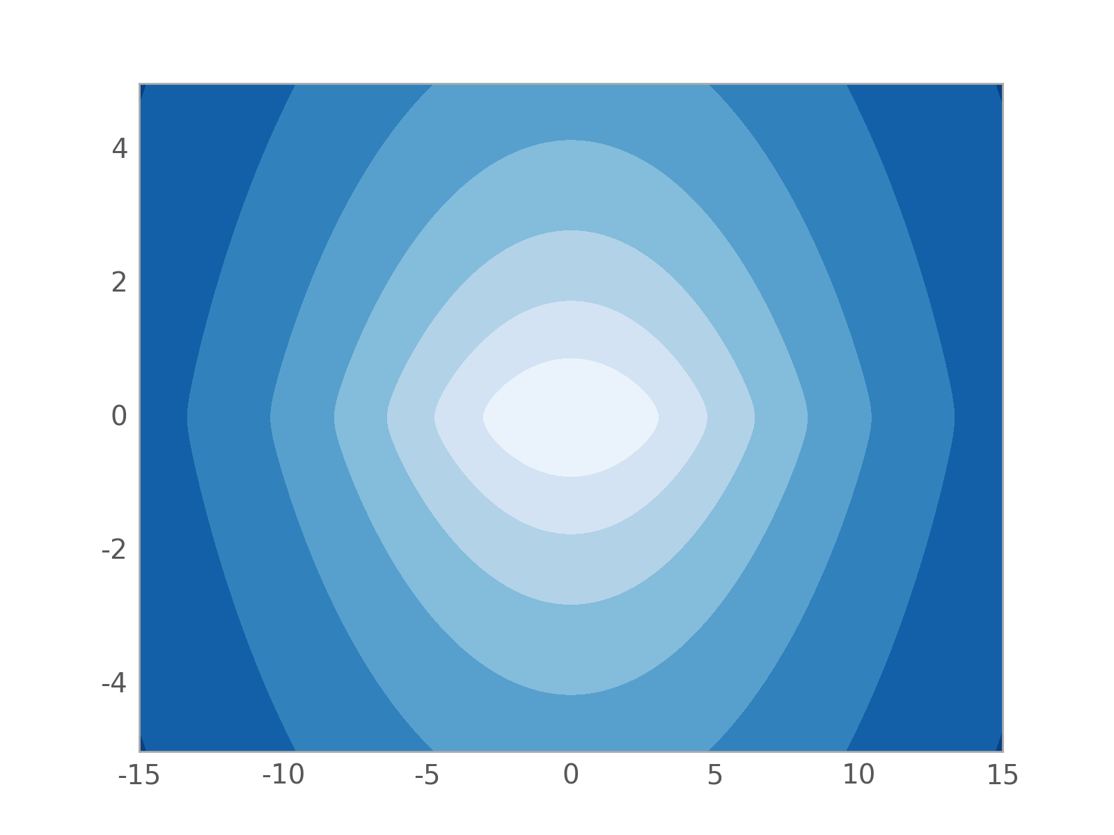
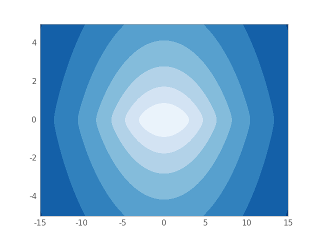
To instead make a 2D contour plot over \(x\) and \(z\) along with \(y=0\), pass in a 1D grid of values for \(x\) and a 1D grid of values for \(z\) (the meshgridding is taken care of internally):
>>> x = np.linspace(-15,15,100)
>>> z = np.linspace(-5,5,100)
>>> p.plot_contours(grid=(x, 1., z))
(Source code, png, hires.png, pdf)
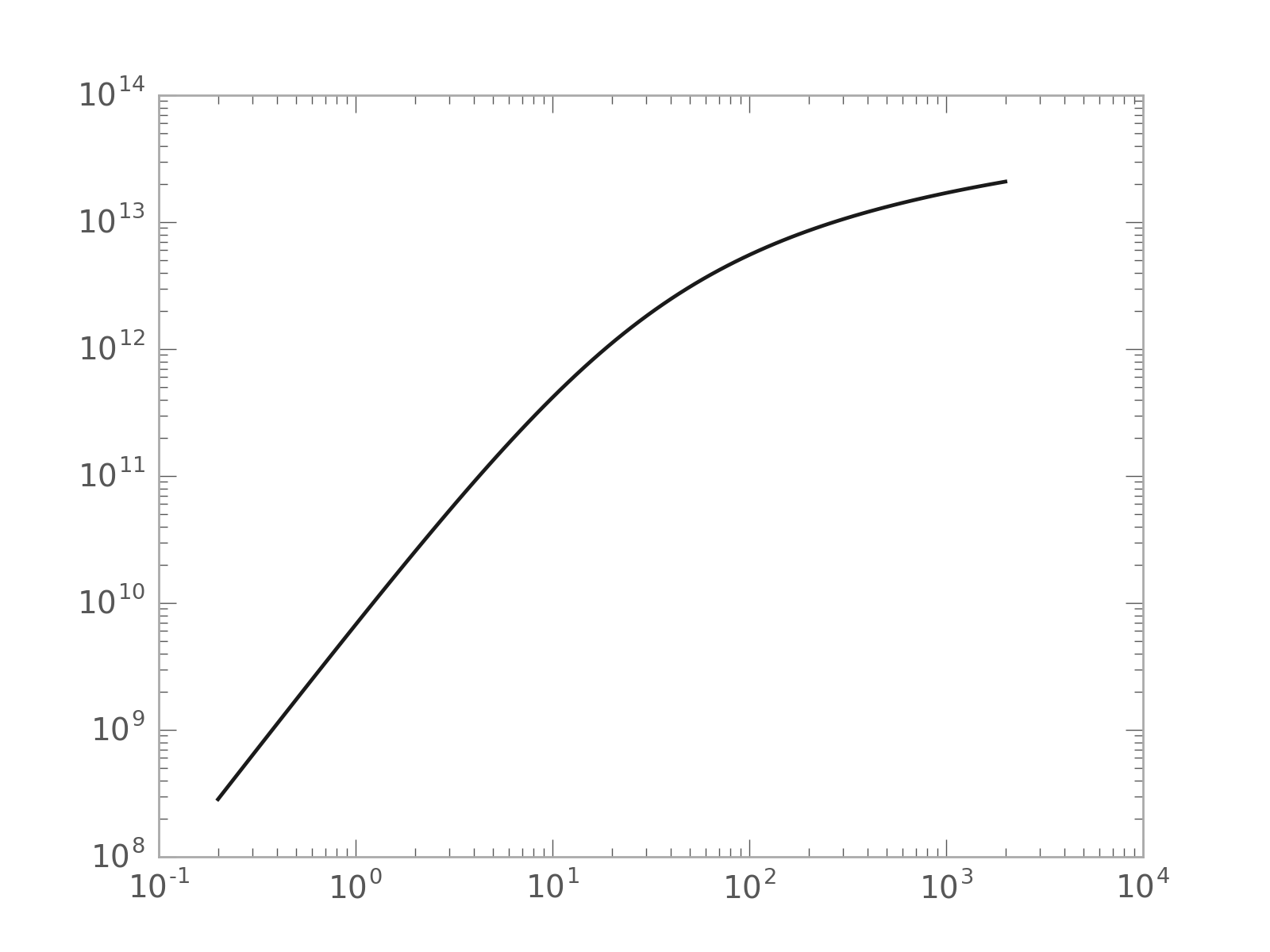
mass_enclosed() is a method that
numerically estimates the mass enclosed within a spherical shell defined
by the specified position. This numerically estimates
\(\frac{d \Phi}{d r}\) along the vector pointing at the specified position
and estimates the enclosed mass simply as
\(M(<r)\approx\frac{r^2}{G} \frac{d \Phi}{d r}\). This function can
be used to compute, for example, a mass profile:
>>> import matplotlib.pyplot as pl
>>> pot = gp.SphericalNFWPotential(v_c=0.5, r_s=20., units=galactic)
>>> pos = np.zeros((3,100))
>>> pos[0] = np.logspace(np.log10(20./100.), np.log10(20*100.), pos.shape[1])
>>> m_profile = pot.mass_enclosed(pos)
>>> pl.loglog(pos, m_profile, marker=None)
(Source code, png, hires.png, pdf)

Potential objects can be pickled
and can therefore be stored for later use. However, pickles are saved as binary
files. It may be useful to save to or load from text-based specifications of
Potential objects. This can be done with gala.potential.save() and
gala.potential.load(), or with the save()
and method:
>>> from gala.potential import load
>>> pot = gp.SphericalNFWPotential(v_c=500*u.km/u.s, r_s=20.*u.kpc,
...                                units=galactic)
>>> pot.save("potential.yml")
>>> load("potential.yml")
<SphericalNFWPotential: v_c=0.51, r_s=20.00 (kpc,Myr,solMass,rad)>
Using gala.potential
More details are provided in the linked pages below:
API
gala.potential Package
Functions
from_equation(expr, vars, pars[, name, hessian]) |
Create a potential class from an expression for the potential. |
load(f[, module]) |
Read a potential specification file and return a PotentialBase object instantiated with parameters specified in the spec file. |
save(potential, f) |
Write a PotentialBase object out to a text (YAML) file. |
Classes
CCompositePotential |
|
CPotentialBase |
A baseclass for defining gravitational potentials implemented in C. |
CompositePotential(*args, **kwargs) |
A potential composed of several distinct components. |
FlattenedNFWPotential(v_c, r_s, q_z, units) |
Flattened NFW potential. |
HarmonicOscillatorPotential(omega[, units]) |
Represents an N-dimensional harmonic oscillator. |
HenonHeilesPotential([units]) |
The Hénon-Heiles potential. |
HernquistPotential(m, c, units) |
Hernquist potential for a spheroid. |
IsochronePotential(m, b, units) |
The Isochrone potential. |
JaffePotential(m, c, units) |
Jaffe potential for a spheroid. |
KeplerPotential(m, units) |
The Kepler potential for a point mass. |
KuzminPotential(m, a, units) |
The Kuzmin flattened disk potential. |
LM10Potential([units, disk, bulge, halo]) |
The Galactic potential used by Law and Majewski (2010) to represent the Milky Way as a three-component sum of disk, bulge, and halo. |
LeeSutoTriaxialNFWPotential(v_c, r_s, a, b, ...) |
Approximation of a Triaxial NFW Potential with the flattening in the density, not the potential. |
LogarithmicPotential(v_c, r_h, q1, q2, q3[, ...]) |
Triaxial logarithmic potential. |
MiyamotoNagaiPotential(m, a, b, units) |
Miyamoto-Nagai potential for a flattened mass distribution. |
PlummerPotential(m, b, units) |
Plummer potential for a spheroid. |
PotentialBase(parameters[, units]) |
A baseclass for defining pure-Python gravitational potentials. |
SphericalNFWPotential(v_c, r_s, units) |
Spherical NFW potential. |
StonePotential(m, r_c, r_h, units) |
Stone potential from Stone & Ostriker (2015). |
Class Inheritance Diagram