Integrate an orbit with uncertainties in Milky Way model

gala provides a simple mass model for the Milky Way based on recent measurements of the enclosed mass compiled from the literature. See the Defining a Milky Way potential model documentation for more information about how this model was defined.

In this example, we will use the position and velocity and uncertainties of the Milky Way satellite galaxy “Draco” to integrate orbits in a Milky Way mass model starting from samples from the error distribution over initial conditions defined by its observed kinematics. We will then compute distributions of orbital properties like orbital period, pericenter, and eccentricity.

Let’s start by importing packages we will need:

# Third-party
import astropy.coordinates as coord
import astropy.units as u
import matplotlib.pyplot as plt
import numpy as np

# Gala
import gala.dynamics as gd
import gala.potential as gp

We will also set the default Astropy Galactocentric frame parameters to the values adopted in Astropy v4.0:

coord.galactocentric_frame_defaults.set("v4.0")

<ScienceState galactocentric_frame_defaults: {'galcen_coord': <ICRS Coordinate: (ra, dec) in deg...>

For the Milky Way model, we’ll use the built-in potential class in gala (see above for definition):

potential = gp.MilkyWayPotential()

For the sky position and distance of Draco, we’ll use measurements from Bonanos et al. 2004. For proper motion components, we’ll use the recent HSTPROMO measurements (Sohn et al. 2017) and the line-of-sight velocity from Walker et al. 2007.

icrs = coord.SkyCoord(
    ra=coord.Angle("17h 20m 12.4s"),
    dec=coord.Angle("+57° 54′ 55″"),
    distance=76 * u.kpc,
    pm_ra_cosdec=0.0569 * u.mas / u.yr,
    pm_dec=-0.1673 * u.mas / u.yr,
    radial_velocity=-291 * u.km / u.s,
)

icrs_err = coord.SkyCoord(
    ra=0 * u.deg,
    dec=0 * u.deg,
    distance=6 * u.kpc,
    pm_ra_cosdec=0.009 * u.mas / u.yr,
    pm_dec=0.009 * u.mas / u.yr,
    radial_velocity=0.1 * u.km / u.s,
)

Let’s start by transforming the measured values to a Galactocentric reference frame so we can integrate an orbit in our Milky Way model. We’ll do this using the velocity transformation support in `astropy.coordinates <http://docs.astropy.org/en/stable/coordinates/velocities.html>`__. We first have to define the position and motion of the sun relative to the Galactocentric frame, and create an `astropy.coordinates.Galactocentric <http://docs.astropy.org/en/stable/api/astropy.coordinates.Galactocentric.html#astropy.coordinates.Galactocentric>`__ object with these parameters. We could specify these things explicitly, but instead we will use the default values that were recently updated in Astropy:

galcen_frame = coord.Galactocentric()
galcen_frame

<Galactocentric Frame (galcen_coord=<ICRS Coordinate: (ra, dec) in deg
    (266.4051, -28.936175)>, galcen_distance=8.122 kpc, galcen_v_sun=(12.9, 245.6, 7.78) km / s, z_sun=20.8 pc, roll=0.0 deg)>

To transform the mean observed kinematics to this frame, we simply do:

galcen = icrs.transform_to(galcen_frame)

That’s it! Now we have to turn the resulting Galactocentric object into orbital initial conditions, and integrate the orbit in our Milky Way model. We’ll use a timestep of 0.5 Myr and integrate the orbit backwards for 10000 steps (5 Gyr):

w0 = gd.PhaseSpacePosition(galcen.data)
orbit = potential.integrate_orbit(w0, dt=-0.5 * u.Myr, n_steps=10000)

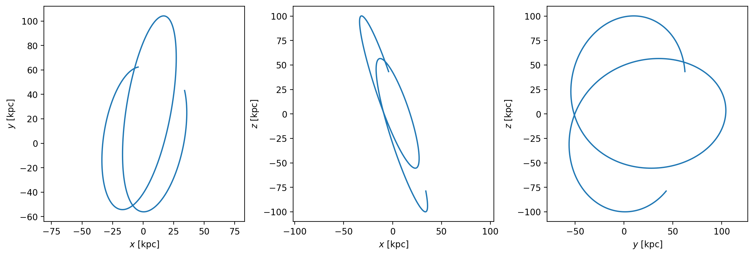
Let’s visualize the orbit:

fig = orbit.plot()

With the orbit object, we can easily compute quantities like the pericenter, apocenter, or eccentricity of the orbit:

orbit.pericenter(), orbit.apocenter(), orbit.eccentricity()

(<Quantity 45.47408489 kpc>,
 <Quantity 105.60902722 kpc>,
 <Quantity 0.39802557>)

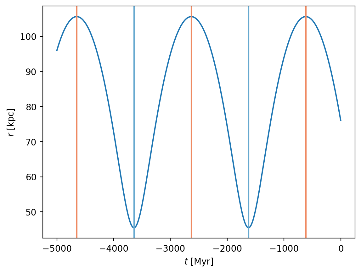
We can also use these functions to get the time of each pericenter or apocenter - let’s plot the time of pericenter, and time of apocenter over the time series of the Galactocentric radius of the orbit:

plt.plot(orbit.t, orbit.spherical.distance, marker="None")

per, per_times = orbit.pericenter(return_times=True, func=None)
apo, apo_times = orbit.apocenter(return_times=True, func=None)

for t in per_times:
    plt.axvline(t.value, color="#67a9cf")

for t in apo_times:
    plt.axvline(t.value, color="#ef8a62")

plt.xlabel("$t$ [{0}]".format(orbit.t.unit.to_string("latex")))
plt.ylabel("$r$ [{0}]".format(orbit.x.unit.to_string("latex")))

Text(0, 0.5, '$r$ [$\\mathrm{kpc}$]')

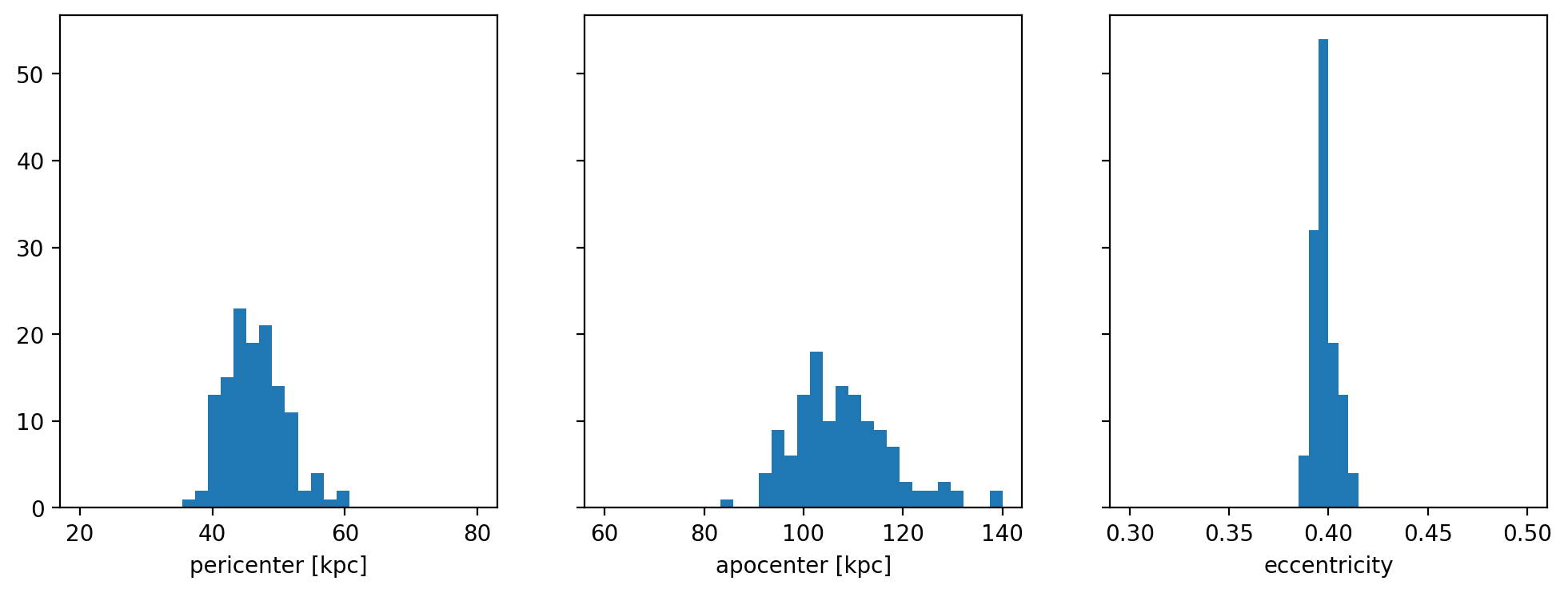
Now we’ll sample from the error distribution over the distance, proper motions, and radial velocity, compute orbits, and plot distributions of mean pericenter and apocenter:

n_samples = 128

dist = (
    np.random.normal(icrs.distance.value, icrs_err.distance.value, n_samples)
    * icrs.distance.unit
)

pm_ra_cosdec = (
    np.random.normal(icrs.pm_ra_cosdec.value, icrs_err.pm_ra_cosdec.value, n_samples)
    * icrs.pm_ra_cosdec.unit
)

pm_dec = (
    np.random.normal(icrs.pm_dec.value, icrs_err.pm_dec.value, n_samples)
    * icrs.pm_dec.unit
)

rv = (
    np.random.normal(
        icrs.radial_velocity.value, icrs_err.radial_velocity.value, n_samples
    )
    * icrs.radial_velocity.unit
)

ra = np.full(n_samples, icrs.ra.degree) * u.degree
dec = np.full(n_samples, icrs.dec.degree) * u.degree

icrs_samples = coord.SkyCoord(
    ra=ra,
    dec=dec,
    distance=dist,
    pm_ra_cosdec=pm_ra_cosdec,
    pm_dec=pm_dec,
    radial_velocity=rv,
)

icrs_samples.shape

(128,)

galcen_samples = icrs_samples.transform_to(galcen_frame)

w0_samples = gd.PhaseSpacePosition(galcen_samples.data)
orbit_samples = potential.integrate_orbit(w0_samples, dt=-1 * u.Myr, n_steps=4000)

orbit_samples.shape

(4001, 128)

peris = orbit_samples.pericenter(approximate=True)

apos = orbit_samples.apocenter(approximate=True)

eccs = orbit_samples.eccentricity(approximate=True)

fig, axes = plt.subplots(1, 3, figsize=(12, 4), sharey=True)

axes[0].hist(peris.to_value(u.kpc), bins=np.linspace(20, 80, 32))
axes[0].set_xlabel("pericenter [kpc]")

axes[1].hist(apos.to_value(u.kpc), bins=np.linspace(60, 140, 32))
axes[1].set_xlabel("apocenter [kpc]")

axes[2].hist(eccs.value, bins=np.linspace(0.3, 0.5, 41))
axes[2].set_xlabel("eccentricity")

Text(0.5, 0, 'eccentricity')