Circular restricted three-body problem#
As a demonstration of the flexibility of the potential clases and reference frame machinery, below we’ll demonstrate how to integrate orbits in the circular restricted three-body problem.
We first need to import some relevant packages:
>>> import astropy.units as u
>>> import matplotlib.pyplot as plt
>>> import numpy as np
>>> from scipy.optimize import root
>>> import gala.integrate as gi
>>> import gala.dynamics as gd
>>> import gala.potential as gp
The “restricted three-body problem” is the problem of solving for the orbit of a test particle interacting with a binary bass system, typically also in the rotating frame of the binary. We’ll assume that the binary consists of a more massive component \(m_1\) and a secondary mass \(m_2\). If the binary components are on circular orbits, and we restict to the plane of motion of the binary, we can change to a rotating reference frame that rotates with the angular frequency of the binary, and cast the problem in terms of scaled units that simplify the expressions and math. In detail, we’ll work in units such that the masses of the two components are \(1 - \mu\) and \(\mu\), where \(\mu = \frac{m_2}{m_1+m_2}\). We’ll also set \(G=1\) and the orbital frequency of the binary to \(\Omega=1\). For more information about the problem setup, see, e.g., this paper.
For our example, we’ll use the value \(\mu = 1/11\), corresponding to a 1:10 mass ratio between the two components of the central binary. In the units defined above, and assuming that the binary components lie on the coordinate \(x\)-axis in the rotating frame, the positions and masses of the two binary components are \(x_1 = -\mu\), \(m_1 = 1-\mu\) and \(x_2 = 1-\mu\), \(m_2 = \mu\), respectively. Let’s start by defining these quantities:
>>> mu = 1/11.
>>> x1 = -mu
>>> m1 = 1-mu
>>> x2 = 1-mu
>>> m2 = mu
Since the potential classes in Gala work with 3-dimensional quantities,
we’ll define the frequency of the binary as a 3D vector:
>>> Omega = np.array([0, 0, 1.])
We’ll now define the gravitational potential of the binary. To do this, we have
to make use of the origin keyword in the potential class initializer to
shift the positions of the component masses to the values defined above. We’ll
store the potentials of the two masses together in a
CCompositePotential:
>>> pot = gp.CCompositePotential()
>>> pot['m1'] = gp.KeplerPotential(m=m1, origin=[x1, 0, 0.])
>>> pot['m2'] = gp.KeplerPotential(m=m2, origin=[x2, 0, 0.])
We now have to define the rotating reference frame:
>>> frame = gp.ConstantRotatingFrame(Omega=Omega)
And finally, we combine the potential and frame into a
Hamiltonian object:
>>> H = gp.Hamiltonian(pot, frame)
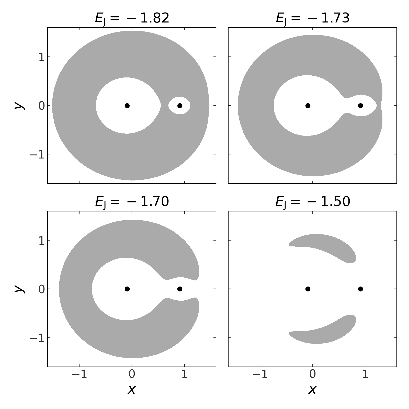
We’re now ready to start integrating orbits! But before we do that, let’s look at the geometry of phase-space to get a sense for what the orbits will look like with different choices of the Jacobi energy. We’ll make a grid of x and y positions and evalutes the Jacobi energy at each position in the grid assuming a zero velocity. We’ll draw filled contours at each value of 4 chosen Jacobi energy values, which will visualize “forbidden regions” of the plane at each value of the Jacobi energy (see Section 3.3.2 in Binney and Tremaine 2008):
>>> grid = np.linspace(-1.75, 1.75, 128)
>>> x_grid, y_grid = np.meshgrid(grid, grid)
>>> xyz = np.vstack((x_grid.ravel(),
...                  y_grid.ravel(),
...                  np.zeros_like(x_grid.ravel())))
>>> Om_cross_x = np.cross(Omega, xyz.T)
>>> E_J = H.potential.energy(xyz) - 0.5*np.sum(Om_cross_x**2, axis=1)
>>> E_J_levels = [-1.82, -1.73, -1.7, -1.5]
(Source code, png, pdf)

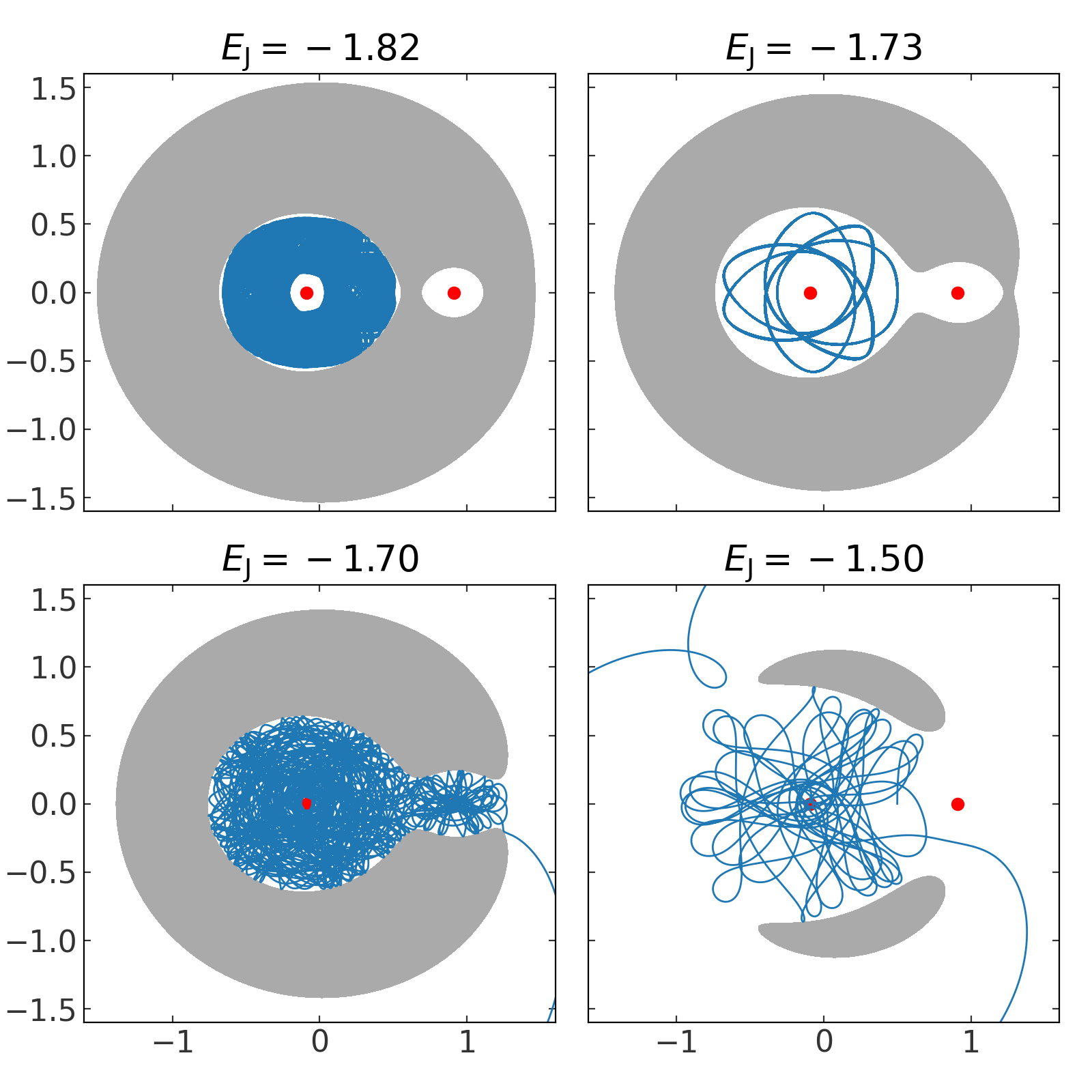
At each of the values of the Jacobi energy chosen above, we’ll now integrate an orbit. To do this, we have to solve for the initial conditions given the Jacobi energy, and convert from rotating frame (Lagrangian) coordinates to canonical coordinates. Let’s define some functions to help with this:
>>> def func_ydot(val, x, H, E_J):
...    ydot = val[0]
...    Om_cross_x = np.cross(H.frame.parameters['Omega'].value, x)
...    eff_pot = H.potential.energy(x).value[0] - 0.5*Om_cross_x.dot(Om_cross_x)
...    return E_J - 0.5*ydot**2 - eff_pot
>>> def xxdot_to_qp(x, xdot, Omega):
...     q = x
...     p = np.array(xdot) + np.cross(Omega, x)
...     return q, p
Now we’ll integrate the orbits at each energy level. We’ll assert that the orbit starts from the y axis at \(x = 0.5\) and solve for the y velocity, \(\dot{y}\), then convert to canonical coordinates:
>>> x0 = [0.5, 0, 0]
>>> orbits = []
>>> for level in E_J_levels:
...     res = root(func_ydot, x0=0.3, args=(x0, H, level))
...     xdot0 = [0, res.x[0], 0.]
...     w0 = np.concatenate(xxdot_to_qp(x0, xdot0, Omega))
...     orbit = H.integrate_orbit(w0, dt=1E-2, n_steps=100000,
...                               Integrator=gi.DOPRI853Integrator)
...     orbits.append(orbit)
(Source code, png, pdf)

