Transforming to actions, angles, and frequencies#
Introduction#
Regular orbits permit a (local) transformation to a set of canonical coordinates such that the momenta are independent, isolating integrals of motion (the actions, \(\boldsymbol{J}\)) and the conjugate coordinate variables (the angles, \(\boldsymbol{\theta}\)) linearly increase with time. Action-angle coordinates are useful for a number of applications because the equations of motion are very simple:
Analytic transformations from phase-space to action-angle coordinates are only known for a few simple cases where the gravitational potential is separable or has many symmetries. However, astronomical systems can often be approximately axisymmetric or triaxial, or have complex radial profiles that are not captured by these simple gravitational potentials where the transformations are known.
Several numerical methods have been developed over recent years to enable approximate transformations between ordinary position and velocity to action-angle coordinates – see [sanders16] for a summary of these methods. In Gala, we have implemented the method described in [sanders14] – later in [sanders16] named the “O2GF” method – for computing actions and angles from numerically integrated orbits. Gala also provides an interface to the galpy implementation of the “Staeckel Fudge” method, which is much faster but only useful for axisymmetric or spherical potentials.
The O2GF action solver#
As mentioned above, this method was first introduced in [sanders14] and later described in [sanders16]. This method is very general in that it works with any numerically-integrated orbital time series. However, it is slower than other approximate methods: If your system is spherical or axisymmetric, other methods will perform much better. If your system is triaxial, this method is your best option. We demonstrate this method below with two qualitatively different orbits:
(see also [binneytremaine] and [mcgill90] for more context). For the examples
below, we will use the galactic unit system and assume the
following imports have been executed:
>>> import astropy.coordinates as coord
>>> import astropy.units as u
>>> import matplotlib.pyplot as plt
>>> import numpy as np
>>> import gala.dynamics as gd
>>> import gala.integrate as gi
>>> import gala.potential as gp
>>> from gala.units import galactic
For many more options for action calculation, see tact.
A tube orbit in an axisymmetric potential#
For an example of an axisymmetric potential, we use a flattened logarithmic potential:
with parameters
For the orbit, we use initial conditions
We first create a potential and set up our initial conditions:
>>> pot = gp.LogarithmicPotential(
...     v_c=150*u.km/u.s, q1=1., q2=1., q3=0.9, r_h=0,
...     units=galactic)
>>> w0 = gd.PhaseSpacePosition(pos=[8, 0, 0.]*u.kpc,
...                            vel=[75, 150, 50.]*u.km/u.s)
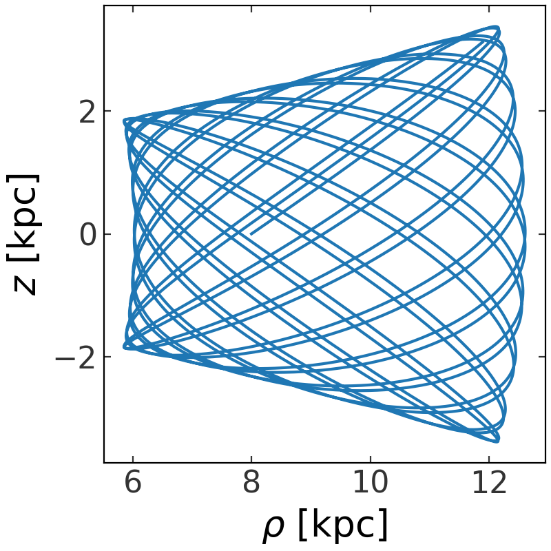
We will now integrate the orbit and plot it in the meridional plane:
>>> w = gp.Hamiltonian(pot).integrate_orbit(w0, dt=0.5, n_steps=10000)
>>> cyl = w.represent_as('cylindrical')
>>> fig = cyl.plot(['rho', 'z'], linestyle='-')
(Source code, png, pdf)

To solve for the actions in the true potential, we first compute the actions in
a “toy” potential – a potential in which we can compute the actions and angles
analytically. The two simplest potentials for which this is possible are the
IsochronePotential and
HarmonicOscillatorPotential. We will use the
Isochrone potential as our toy potential for tube orbits and the harmonic
oscillator for box orbits.
We start by finding the parameters of the toy potential (Isochrone in this case) by minimizing the dispersion in energy for the orbit:
>>> toy_potential = gd.fit_isochrone(w)
>>> toy_potential
<IsochronePotential: m=1.24e+11, b=4.02 (kpc,Myr,solMass,rad)>
The actions and angles in this potential are not the true actions, but will only serve as an approximation. This can be seen in the angles: the orbit in the true angles would be perfectly straight lines with slope equal to the frequencies. Instead, the orbit is wobbly in the toy potential angles:
>>> toy_actions,toy_angles,toy_freqs = toy_potential.action_angle(w)
>>> fig,ax = plt.subplots(1,1,figsize=(5,5))
>>> ax.plot(toy_angles[0], toy_angles[2], linestyle='none', marker=',')
>>> ax.set_xlim(0,2*np.pi)
>>> ax.set_ylim(0,2*np.pi)
>>> ax.set_xlabel(r"$\theta_1$ [rad]")
>>> ax.set_ylabel(r"$\theta_3$ [rad]")
(Source code, png, pdf)

This can also be seen in the value of the action variables, which are not time-independent in the toy potential:
>>> fig,ax = plt.subplots(1,1)
>>> ax.plot(w.t, toy_actions[0], marker='')
>>> ax.set_xlabel(r"$t$ [Myr]")
>>> ax.set_ylabel(r"$J_1$ [rad]")
(Source code, png, pdf)
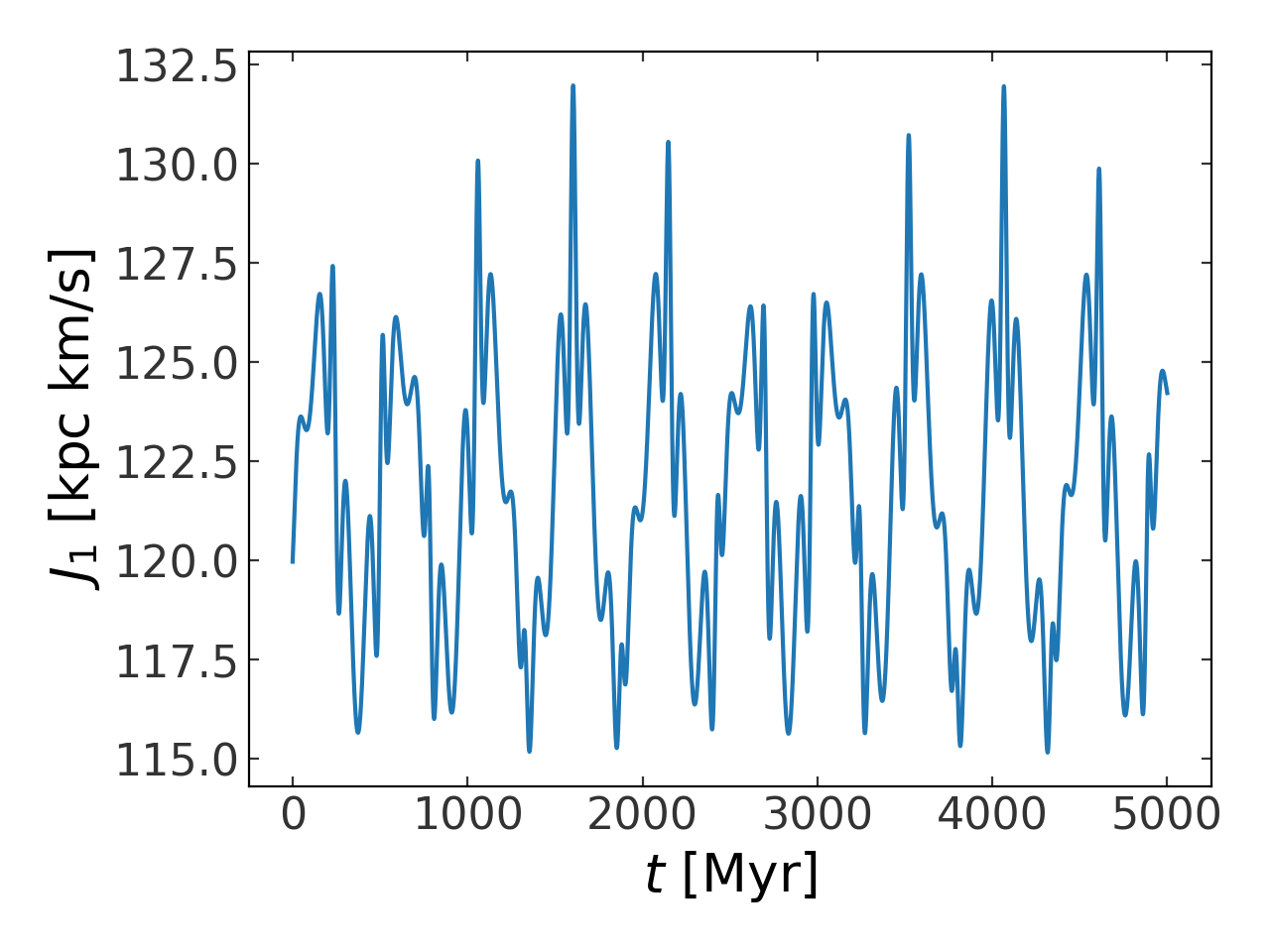

We can now find approximations to the actions in the true potential. We have to
choose the maximum integer vector norm, N_max, which here we arbitrarily set
to 8. This will change depending on the convergence of the action correction
(the properties of the orbit and potential) and the accuracy desired:
>>> result = gd.find_actions_o2gf(w, N_max=8, toy_potential=toy_potential)
>>> result.keys()
dict_keys(['Sn', 'nvecs', 'freqs', 'dSn_dJ', 'angles', 'actions'])
The value of the actions, frequencies, and the angles at t=0 are returned in the result dictionary:
>>> result['actions']
<Quantity [ 0.12472277, 1.22725461, 0.05847431] kpc2 solMass / Myr>
To visualize how the actions are computed, we again plot the actions in the toy potential and then plot the “corrected” actions – the approximation to the actions computed using this machinery:
>>> nvecs = gd.generate_n_vectors(8, dx=1, dy=2, dz=2)
>>> act_correction = nvecs.T[...,None] * result['Sn'][None,:,None] * np.cos(nvecs.dot(toy_angles))[None]
>>> action_approx = toy_actions - 2*np.sum(act_correction, axis=1)*u.kpc**2/u.Myr
>>>
>>> fig,ax = plt.subplots(1,1)
>>> ax.plot(w.t, toy_actions[0].to(u.km/u.s*u.kpc), marker='', label='$J_1$')
>>> ax.plot(w.t, action_approx[0].to(u.km/u.s*u.kpc), marker='', label="$J_1'$")
>>> ax.set_xlabel(r"$t$ [Myr]")
>>> ax.set_ylabel(r"[kpc ${\rm M}_\odot$ km/s]")
>>> ax.legend()
(Source code, png, pdf)
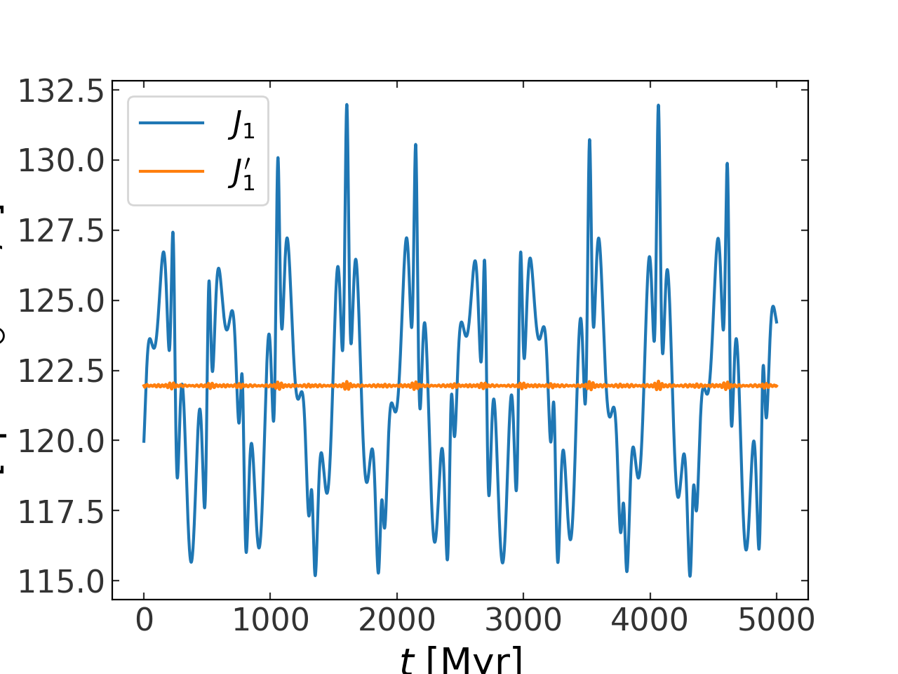

Above the blue line represents the approximation of the actions in the true potential.
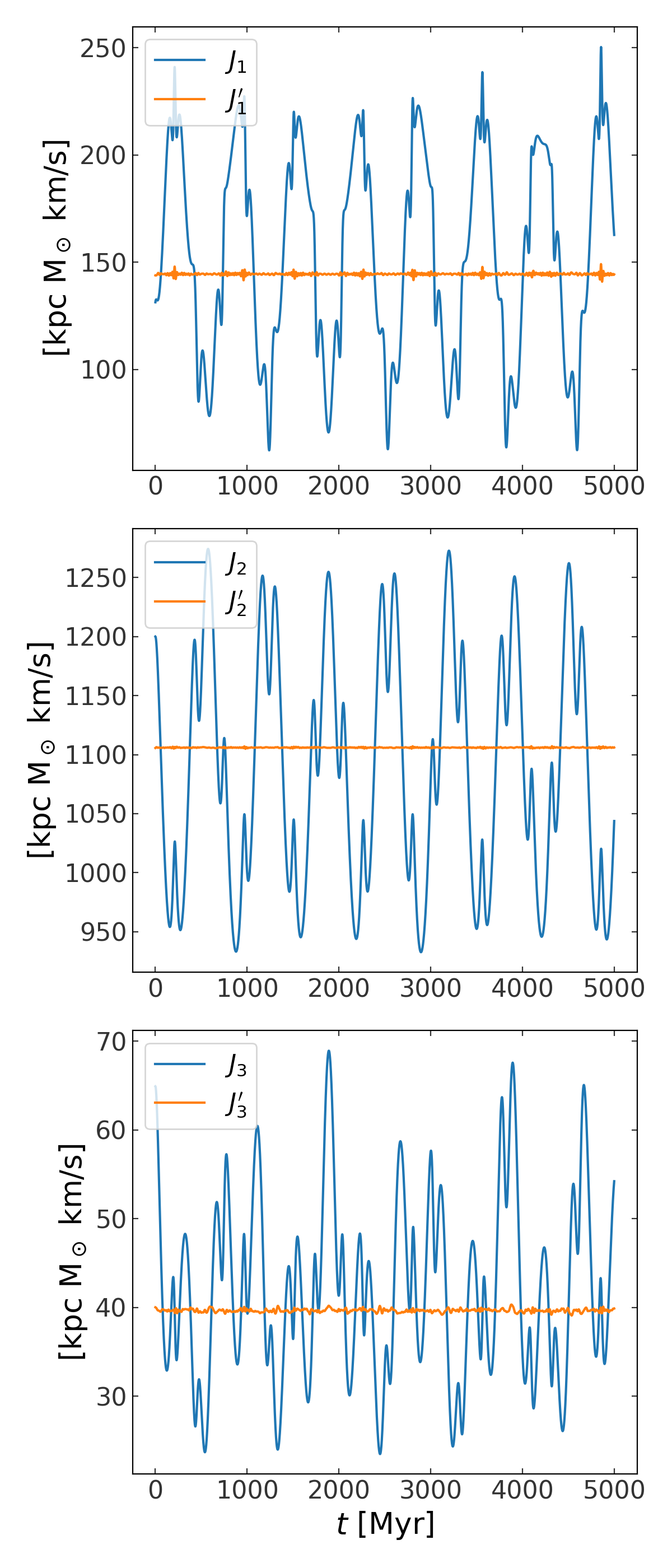
A tube orbit in a triaxial potential#
The same procedure works for regular orbits in more complex potentials. We demonstrate this below by repeating the above in a triaxial potential. We again use a logarithmic potential, but with flattening along two dimensions:
with parameter values:
and the same initial conditions as above:
import astropy.coordinates as coord
import astropy.units as u
import matplotlib.pyplot as plt
import numpy as np
import gala.potential as gp
import gala.dynamics as gd
from gala.units import galactic

# define potential
pot = gp.LogarithmicPotential(v_c=150*u.km/u.s, q1=1., q2=0.9, q3=0.8, r_h=0,
                              units=galactic)

# define initial conditions
w0 = gd.PhaseSpacePosition(pos=[8, 0, 0.]*u.kpc,
                           vel=[75, 150, 50.]*u.km/u.s)

# integrate orbit
w = gp.Hamiltonian(pot).integrate_orbit(w0, dt=0.5, n_steps=10000)

# solve for toy potential parameters
toy_potential = gd.fit_isochrone(w)

# compute the actions,angles in the toy potential
toy_actions,toy_angles,toy_freqs = toy_potential.action_angle(w)

# find approximations to the actions in the true potential
import warnings
with warnings.catch_warnings(record=True):
    warnings.simplefilter("ignore")
    result = gd.find_actions_o2gf(w, N_max=8, toy_potential=toy_potential)

# for visualization, compute the action correction used to transform the
#   toy potential actions to the approximate true potential actions
nvecs = gd.generate_n_vectors(8, dx=1, dy=2, dz=2)
act_correction = nvecs.T[...,None] * result['Sn'][0][None,:,None] * np.cos(nvecs.dot(toy_angles))[None]
action_approx = toy_actions - 2*np.sum(act_correction, axis=1)*u.kpc**2/u.Myr

fig,axes = plt.subplots(3,1,figsize=(6,14))

for i,ax in enumerate(axes):
    ax.plot(w.t, toy_actions[i].to(u.km/u.s*u.kpc), marker='', label='$J_{}$'.format(i+1))
    ax.plot(w.t, action_approx[i].to(u.km/u.s*u.kpc), marker='', label="$J_{}'$".format(i+1))
    ax.set_ylabel(r"[kpc ${\rm M}_\odot$ km/s]")
    ax.legend(loc='upper left')

ax.set_xlabel(r"$t$ [Myr]")
fig.tight_layout()
(Source code, png, pdf)
Using the Staeckel Fudge in Galpy#
Gala can transform its Orbit and Potential objects into Galpy Orbit and Potential objects, making it possible to easily use the “Staeckel Fudge” [binney12] implementation in Galpy. This method, as
implemented, is only applicable for axisymmetric systems, but is much faster
than the O2GF method for estimating actions, angles, and frequencies from
phase-space positions. As an example of this functionality, below we will
compute the vertical frequency as a function of action for a grid of orbits in a
two-component model for a galactic potential (a disk + halo model).
We will start by defining the potential model:
>>> halo = gp.NFWPotential.from_M200_c(
...     M200=1e12*u.Msun, c=15,
...     units=galactic
... )
>>> disk = gp.MN3ExponentialDiskPotential(
...     m=8e10*u.Msun, h_R=3.5*u.kpc, h_z=0.4*u.kpc,
...     units=galactic
... )
>>> pot = halo + disk
We next define a grid of orbital initial conditions with close to the circular velocity but varying vertical velocities:
>>> vcirc = pot.circular_velocity([8, 0, 0])
>>> vz_grid = np.linspace(0.5, 200, 64) * u.km/u.s
>>> xyz = np.repeat([[8., 0, 0]], len(vz_grid), axis=0).T * u.kpc
>>> vxyz = np.repeat([[0, 1.1, 0]], len(vz_grid), axis=0).T * vcirc
>>> vxyz[2] = vz_grid
>>> w0 = gd.PhaseSpacePosition(xyz, vxyz)
We can now integrate these orbits in the total potential. Note that we can specify the integrator using a string name:
>>> orbits = pot.integrate_orbit(
... w0, dt=1, t1=0, t2=4*u.Gyr,
... Integrator='dopri853'
... )
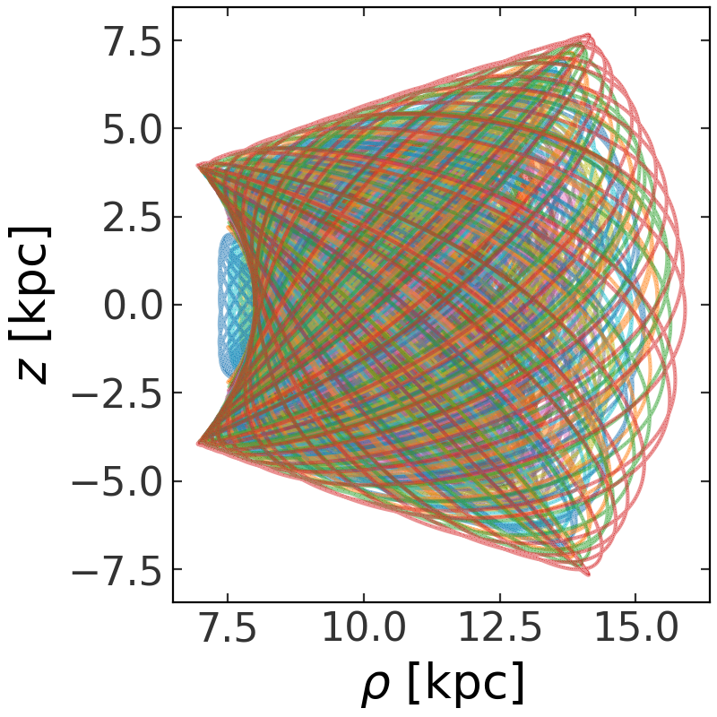
>>> orbits.cylindrical.plot(['rho', 'z'], alpha=0.5, marker=',')
(Source code, png, pdf)

With the orbits in hand, we can compute the approximate actions, angles, and frequencies with the Staeckel Fudge using Galpy (for more information, see the Galpy documentation):
>>> from gala.dynamics.actionangle import get_staeckel_fudge_delta
>>> from galpy.actionAngle import actionAngleStaeckel
>>> galpy_potential = pot.as_interop("galpy")
>>> J = np.zeros((3, orbits.norbits))
>>> Omega = np.zeros((3, orbits.norbits))
>>> for n, orbit in enumerate(orbits.orbit_gen()):
...     o = orbit.to_galpy_orbit()
...     delta = get_staeckel_fudge_delta(pot, orbit)
...     staeckel = actionAngleStaeckel(pot=galpy_potential, delta=delta)
...     af = staeckel.actionsFreqs(o)
...     af = np.mean(np.stack(af), axis=1)
...     J[:3, n] = af[:3]
...     Omega[:3, n] = af[3:]
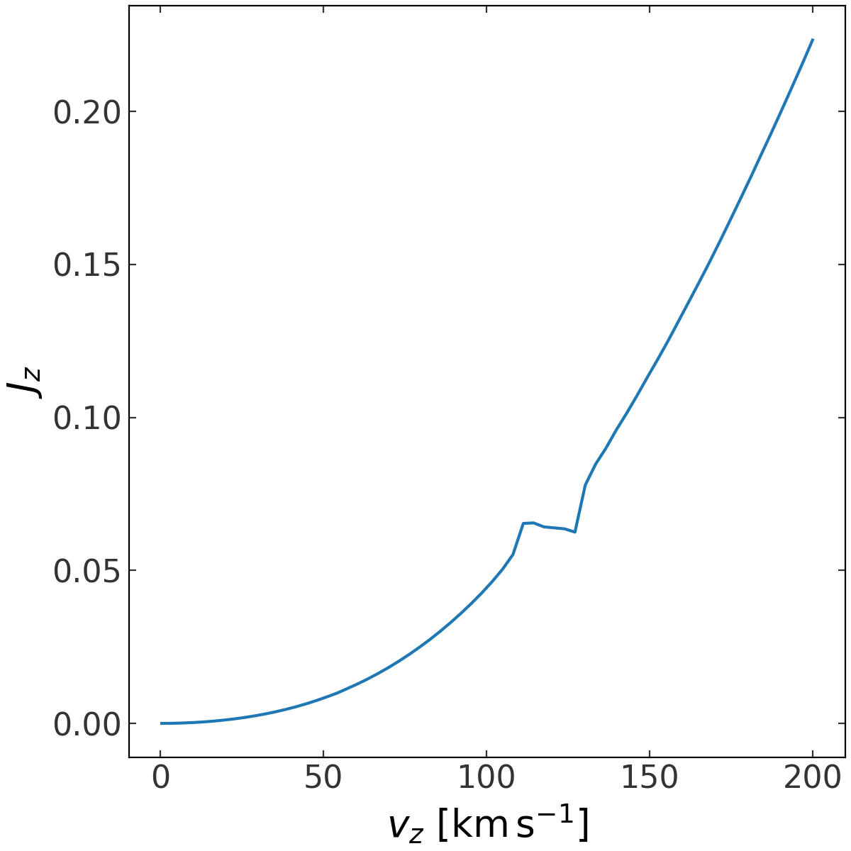
Let’s visualize the dependence of the vertical action on the value of the vertical velocity we used as initial conditions:
>>> plt.plot(w0.v_z, J[2])
(Source code, png, pdf)

The overall trend looks right, but what is that weird break that occurs around \(v_z\) ~ 120 km/s? Let’s visualize orbits with initial conditions just next to and within this region:
>>> i1 = np.abs(w0.v_z.value - 120).argmin()
>>> i2 = np.abs(w0.v_z.value - 100).argmin()
>>> orbits[:, i1].cylindrical.plot(['rho', 'z'], alpha=0.5, marker=',')
>>> orbits[:, i2].cylindrical.plot(['rho', 'z'], alpha=0.5, marker=',')
(Source code, png, pdf)
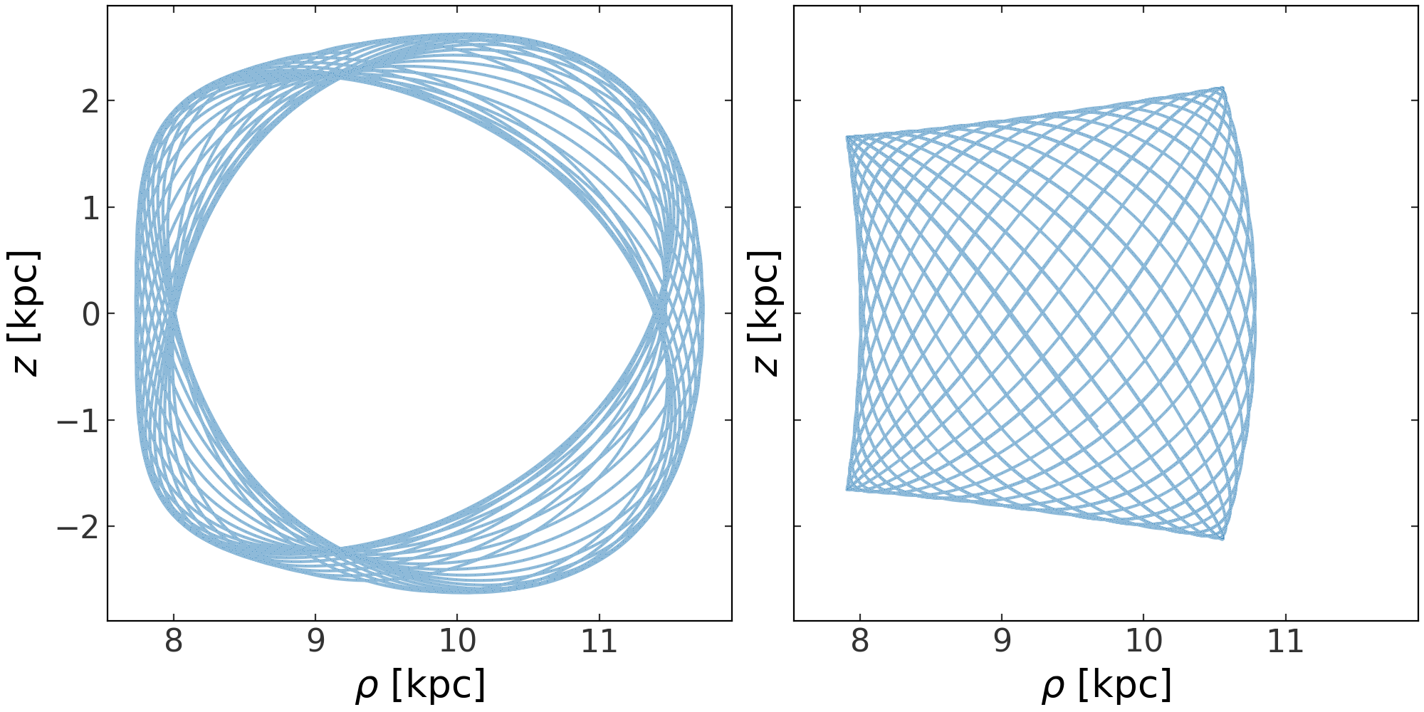
Aha! This region is special: it is a resonance in the potential. Orbits in this region of phase-space have qualitatively different behavior than those outside of this region because they are trapped by the resonance. For these orbits, where strong potential resonances occur, the Staeckel Fudge approximation will return incorrect and potentially misleading action, angle, and frequency values.
References#
Binney (2012) Actions for axisymmetric potentials
Sanders & Binney (2014) Actions, angles and frequencies for numerically integrated orbits
Sanders & Binney (2016) A review of action estimation methods for galactic dynamics
Binney & Tremaine (2008) Galactic Dynamics
McGill & Binney (1990) Torus construction in general gravitational potentials