What’s New in gala v1.0?#
Overview#
Gala 1.0 is a major release with significant new functionality (some of which is described below).
This release includes (among other things):
Great circle coordinate systems#
Great circle coordinate frames (GCFs) are heliocentric coordinate systems that are
typically specified as a rotation away from standard equatorial ICRS
coordinates. The resulting longitude and latitude components of a GCF specify
the angle along the great circle and the angle perpendicular (in gala, we use
\(\phi_1\) / phi1 to represent the longitude, and \(\phi_2\) /
phi2 to represent the latitude). These frames are typically defined by
specifying the coordinate of the pole of the great circle, and either the
origin, \((\phi_1, \phi_2) = (0, 0)\), or the longitude of the old system
(i.e. ICRS) to put at longitude \(\phi_1 = 0\) in the new frame. The new
GreatCircleICRSFrame supports both of these options, along with two other
possible ways for defining a GCF: by specifying two points along the great
circle in the old frame, and by directly specifying the cartesian basis of the
GCF in the old coordinate system. For example, to create a GCF from a pole and
longitude zero-point:
>>> import astropy.units as u
>>> from astropy.coordinates import SkyCoord
>>> from gala.coordinates import GreatCircleICRSFrame
>>> pole = SkyCoord(ra=255*u.deg, dec=-11.5*u.deg)
>>> gcf = GreatCircleICRSFrame(pole=pole, ra0=170*u.deg)
Or, to create a GCF from two endpoints along a great circle:
>>> pt1 = SkyCoord(ra=170.*u.deg, dec=23.18*u.deg)
>>> pt2 = SkyCoord(ra=125.7*u.deg, dec=-72.2*u.deg)
>>> gcf2 = GreatCircleICRSFrame.from_endpoints(pt1, pt2)
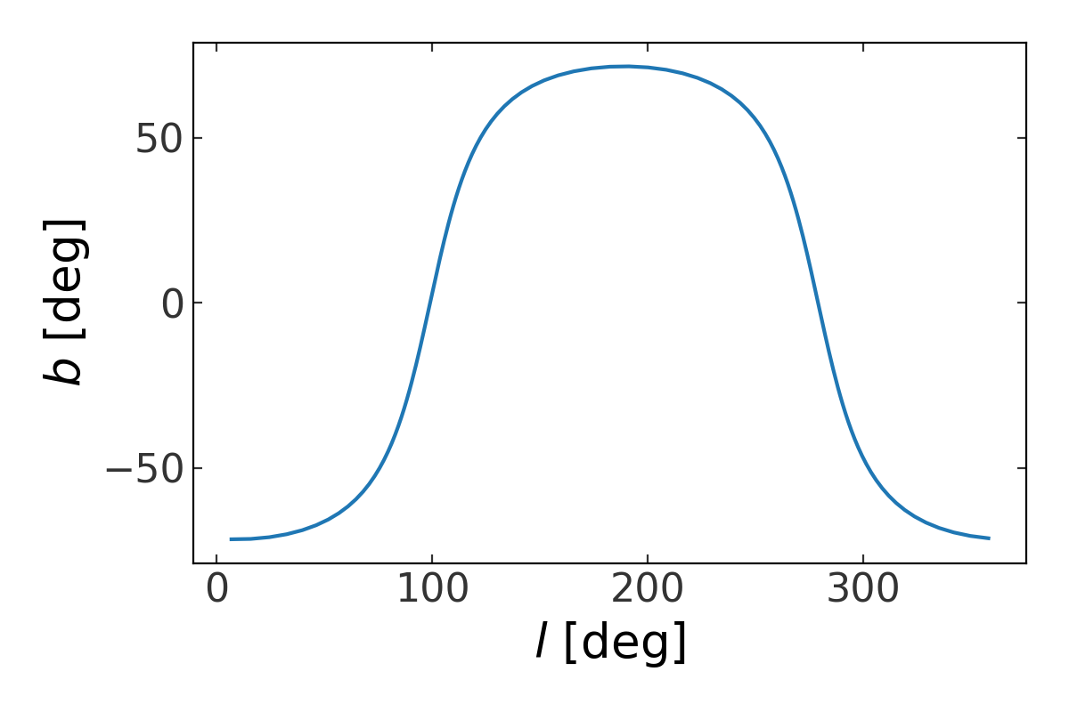
However you define a great circle frame, these can be used with the Astropy coordinate transformation machinery to transform positions and velocity components to and from this and other coordinate frames. For example, to transform a grid of points along latitude=0 in one of these systems to Galactic coordinates to plot the great circle on the sky, we can do:
>>> import numpy as np
>>> grid_c = SkyCoord(phi1=np.linspace(0, 360, 128)*u.deg, phi2=0*u.deg,
...                   frame=gcf2)
>>> grid_c = grid_c.galactic
When plotted, this would show the track of the great circle in Galactic coordinates, i.e.:
(Source code, png, pdf)
New potential models, including MWPotential2014#
Gala now contains an implementation of the Galpy / Bovy 2015
MWPotential2014, here called BovyMWPotential2014. This
potential class can be used like any other potential object in Gala, for
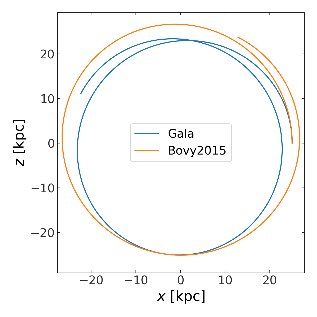
example, for orbit integration. As a brief demo, here we compare the orbit of a
Milky Way halo object in BovyMWPotential2014 as compared to
the default Gala Milky Way model implemented as
MilkyWayPotential:
>>> import gala.dynamics as gd
>>> import gala.potential as gp
>>> mw_gala = gp.MilkyWayPotential()
>>> mw_bovy = gp.BovyMWPotential2014()
>>> w0 = gd.PhaseSpacePosition(pos=[25., 0, 0]*u.kpc,
...                            vel=[0, 0, 200.]*u.km/u.s)
>>> orbit_gala = mw_gala.integrate_orbit(w0, dt=1., n_steps=1000)
>>> orbit_bovy = mw_bovy.integrate_orbit(w0, dt=1., n_steps=1000)
Here is a comparison of the two orbits over-plotted on the same axes:
(Source code, png, pdf)
Basis function expansion potential models with the self-consistent field method#
Gala now contains support for constructing and using flexible (static) gravitational potential models using the self-consistent field (SCF) basis function expansion method. Expansion coefficients can be computed from both analytic density distributions or from discrete particle distributions (e.g., from an N-body simulation). For more information about this new subpackage, see the Self-consistent field (SCF) documentation.
Stellar stream coordinate frame names now reflect the source reference#
Each of the stellar stream coordinate frames now contains the name of the author
that defined the frame. For example, the GD1 frame has been renamed to
GD1Koposov10 to indicate that the frame was defined in
Koposov et al. 2010. This is true for each of the major stellar stream frames:
GD1has been renamedGD1Koposov10Sagittariushas been renamedSagittariusLaw10Orphanhas been renamedOrphanNewberg10, and a new Orphan stream coordinate frame has been added:OrphanKoposov19Ophiuchushas been renamedOphiuchusPriceWhelan16Pal5has been renamedPal5PriceWhelan18MagellanicStreamhas been renamedMagellanicStreamNidever08
Transforming proper motion covariance matrices#
The Gaia mission provides full astrometric covariance matrices for each of its
sources, which not only specify the uncertainty in each parameter, but also
specify the correlations between the uncertainties of the astrometric
parameters. These covariance matrices are provided in the ICRS coordinate
system, but often it is useful to transform the Gaia data to other coordinate
systems when, e.g., modeling stellar streams. The proper motion covariance
matrix can be analytically and straightforwardly transformed along with the
positions and proper motions themselves if the transformation is a rotation away
from ICRS, such as the case for the new GreatCircleICRSFrame or stellar
stream coordinate frames described above. As an example, we will transform the
Gaia proper motion covariance matrix for a source to the GD1Koposov10
coordinate frame:
>>> from gala.coordinates import transform_pm_cov, GD1Koposov10
>>> cov = np.array([[ 0.07567177, -0.01698125],
...                 [-0.01698125,  0.03907039]])
>>> c = SkyCoord(ra=130.99*u.deg, dec=34.53*u.deg,
...              distance=454.76*u.pc,
...              pm_ra_cosdec=11.5*u.mas/u.yr,
...              pm_dec=-23.46661*u.mas/u.yr)
>>> cov_gd1 = transform_pm_cov(c, cov, GD1Koposov10)