Examples#
For the examples below the following imports have already been executed:
import astropy.units as u
import matplotlib as mpl
import matplotlib.pyplot as plt
import numpy as np
from gala.potential import scf
Computing expansion coefficients from particle positions#
To compute expansion coefficients for a distribution of particles or discrete
samples from a density distribution, use
compute_coeffs_discrete. In this example, we will generate
particle positions from a Plummer density profile, compute the expansion
coefficients assuming spherical symmetry, then re-compute the expansion
coefficients and variances (Weinberg 1996; [W96]) allowing for non-spherical
terms (e.g., \(l,m>0\)).
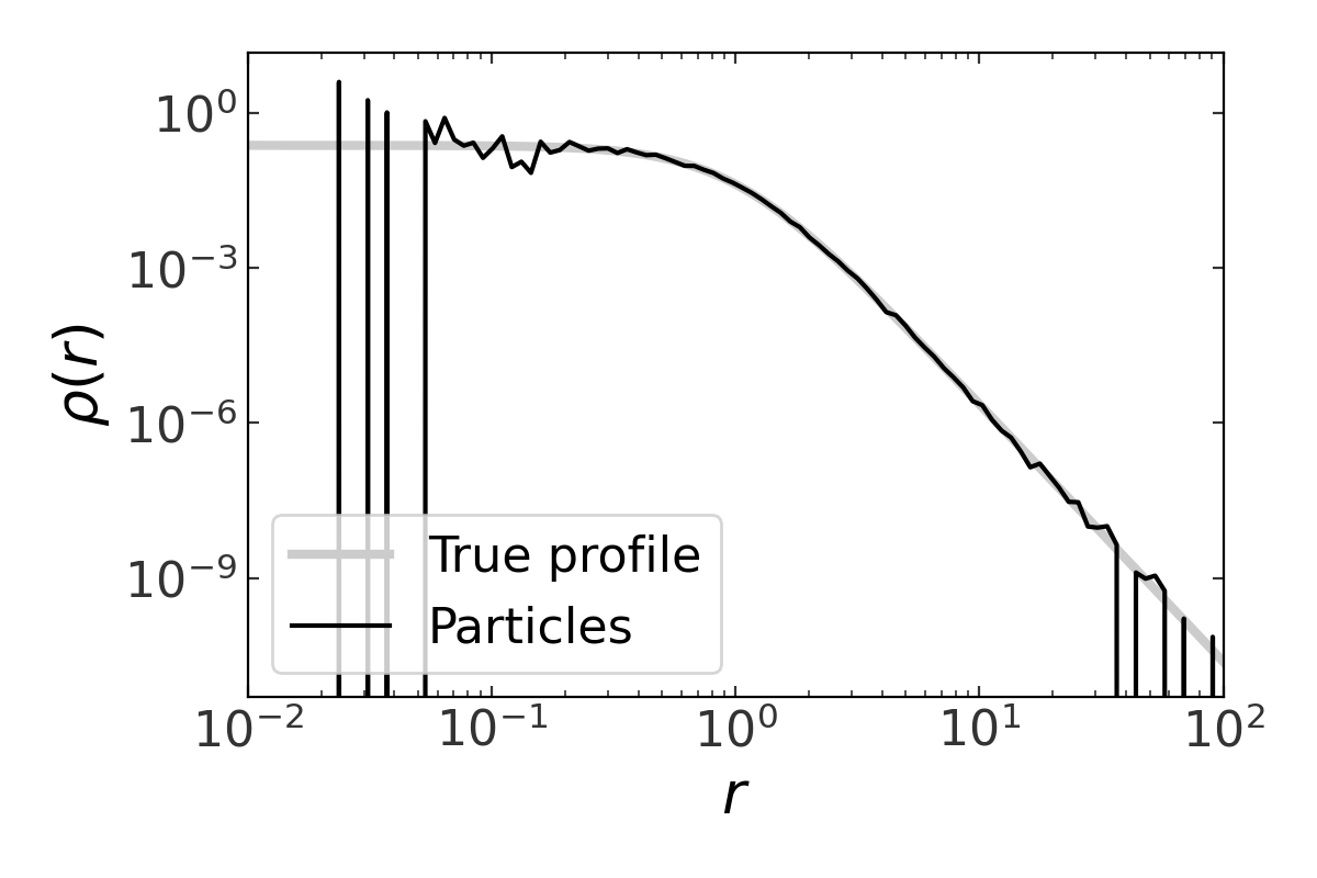
We’ll start by generating samples from a Plummer sphere (see Section 3 of [HMV11] for more details). To do this, we will use inverse transform sampling by inverting the cumulative mass function (in this case, the mass enclosed):
For simplicity, we will work with units in which \(a=1\) and \(M=1\). To generate radii, we first randomly generate values of \(\mu\) uniformly distributed between 0 and 1, then compute the value of \(r\) for each sample; the radii will then be distributed following a Plummer profile. For this example, we’ll use 16384 samples:
def sample_r(size=1):
    mu = np.random.random(size=size)
    return 1 / np.sqrt(mu**(-2/3) - 1)

n_samples = 16384
r = sample_r(size=n_samples)
Let’s plot the density profile derived from these samples vs. the true profile:

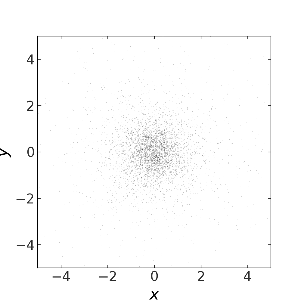
With the above, we now have sampled spherical radii that follow the desired density profile. To compute the expansion coefficients needed to represent this density using SCF with Hernquist radial functions, we first need to convert to 3D cartesian positions. We will distribute these particles uniformly in angles:
phi = np.random.uniform(0, 2*np.pi, size=n_samples)
theta = np.arccos(2*np.random.random(size=n_samples) - 1)

xyz = np.zeros((n_samples, 3))
xyz[:,0] = r * np.cos(phi) * np.sin(theta)
xyz[:,1] = r * np.sin(phi) * np.sin(theta)
xyz[:,2] = r * np.cos(theta)

plt.figure(figsize=(5,5))
plt.plot(xyz[:,0], xyz[:,1], linestyle='none',
         marker=',', alpha=0.25, color='k')
plt.xlim(-5, 5)
plt.ylim(-5, 5)
plt.xlabel('$x$')
plt.ylabel('$y$')
(Source code, png, pdf)
To compute the expansion coefficients, we then pass the positions xyz and
masses of each “particle” to compute_coeffs_discrete. We
will generate an array of masses that sum to 1, per our choice of units above.
To start, we’ll assume that the particle distribution has spherical symmetry and
ignore terms with \(l>0\). We’ll then plot the magnitude of the coefficients
as a function of \(n\) (but we’ll ignore the sine terms, \(T_{nlm}\) for
this example):
mass = np.ones(n_samples) / n_samples
S,T = scf.compute_coeffs_discrete(xyz, mass=mass, nmax=16, lmax=0, r_s=1.)

plt.semilogy(np.abs(S[:,0,0]), marker=None, lw=2)
plt.xlabel("$n$")
plt.ylabel("$S_{n00}$")
plt.tight_layout()
(Source code, png, pdf)

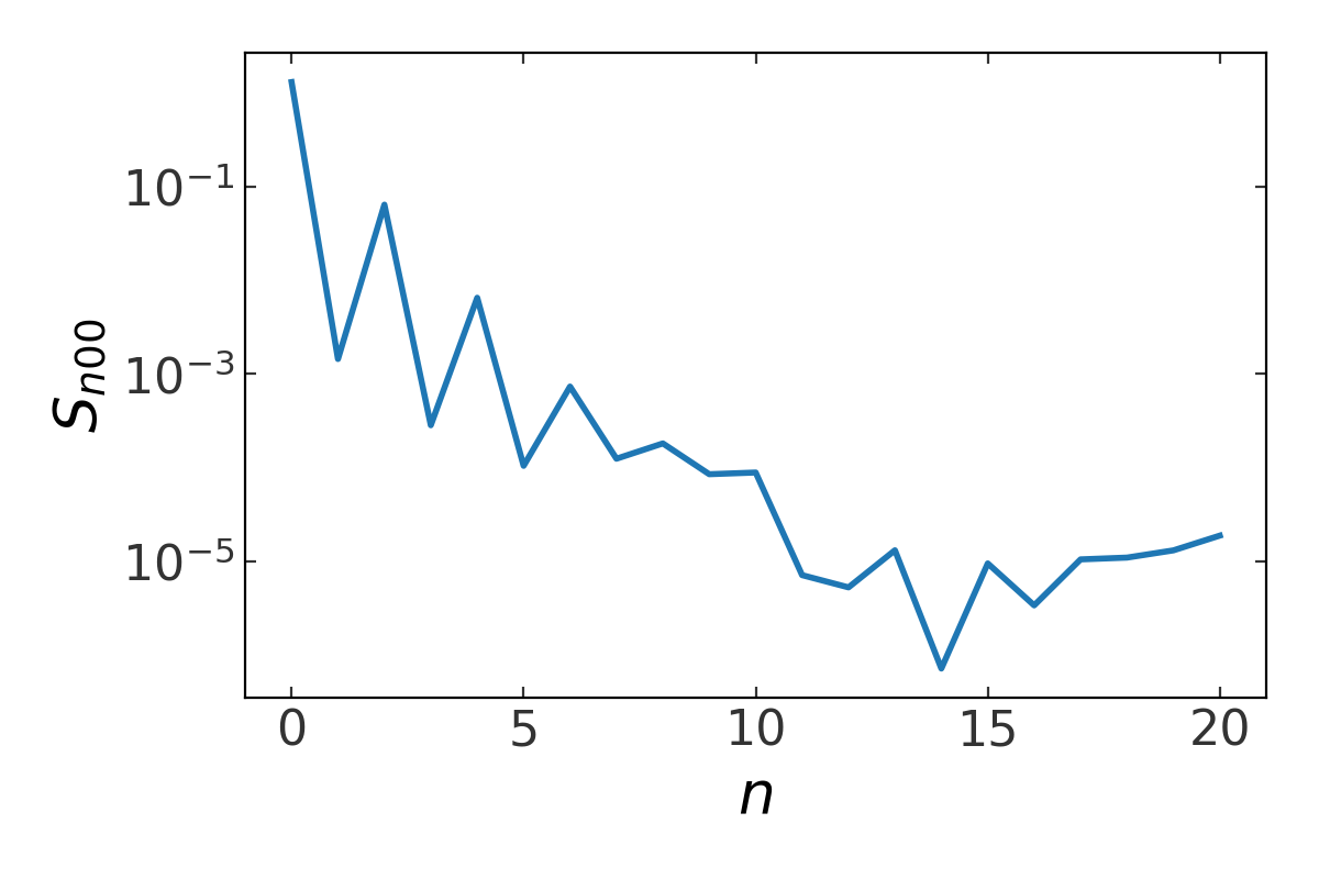
In addition to computing the coefficient values, we can also compute the variances of the coefficients. Here we will relax the assumption about spherical symmetry by setting \(l_{\rm max}=4\). By computing the variance of each coefficient, we can estimate the signal-to-noise ratio of each expansion term and use this to help decide when to truncate the expansion (see [W96] for the methodology and reasoning behind this):
S, T, Cov = scf.compute_coeffs_discrete(
    xyz, mass=mass, r_s=1.,
    nmax=10, lmax=4, skip_m=True,
    compute_var=True
)

signal_to_noise = np.sqrt(S**2 / Cov[0, 0])

for l in range(S.shape[1]):
    plt.semilogy(signal_to_noise[:,l,0], marker=None, lw=2,
                 alpha=0.5, label='l={}'.format(l))

plt.axhline(1., linestyle='dashed')
plt.xlabel("$n$")
plt.ylabel("$S/N$")
plt.legend()
(Source code, png, pdf)
The horizontal line in the plot above is for a signal-to-noise ratio of 1 – any coefficients with a SNR near or below this line are suspect and likely just adding noise to the expansion. Note that all of the SNR values for \(l > 0\) hover around 1 – this is a good indication that we only need the \(l=0\) terms to accurately represent the density distribution of the particles.
Computing expansion coefficients for an analytic density#
To compute expansion coefficients for an analytic density profile, use
compute_coeffs. In this example, we will write a function
to evaluate an oblate density distribution and compute the expansion
coefficients.
We’ll use a flattened Hernquist profile as our density profile:
In code:
def hernquist_density(r, M, a):
    return M*a / (2*np.pi) / (r*(r+a)**3)

def flattened_hernquist_density(x, y, z, M, a, q):
    s = np.sqrt(x**2 + y**2 + (z/q)**2)
    return hernquist_density(s, M, a)
The function to evaluate the density must take at least 3 arguments: the
cartesian coordinates x, y, z.
We’ll again set \(M=a=1\) and we’ll use a flattening \(q=0.8\). Let’s visualize this by plotting isodensity contours in the \(x\)-\(z\) plane:
(Source code, png, pdf)

To compute the expansion coefficients, we pass the
flattened_hernquist_density() function in to
compute_coeffs. Because this is an axisymmetric density,
we will ignore terms with \(m>0\) by setting skip_m=True:
M = 1.
a = 1.
q = 0.8
coeff = scf.compute_coeffs(flattened_hernquist_density, nmax=8, lmax=8,
                            M=M, r_s=a, args=(M,a,q), skip_m=True)
(S,Serr),(T,Terr) = coeff
Computing the coefficients involves a numerical integration that uses
scipy.integrate.quad, which simultaneously estimates the error in the computed
integral. compute_coeffs returns the coefficient arrays
and these error estimates.
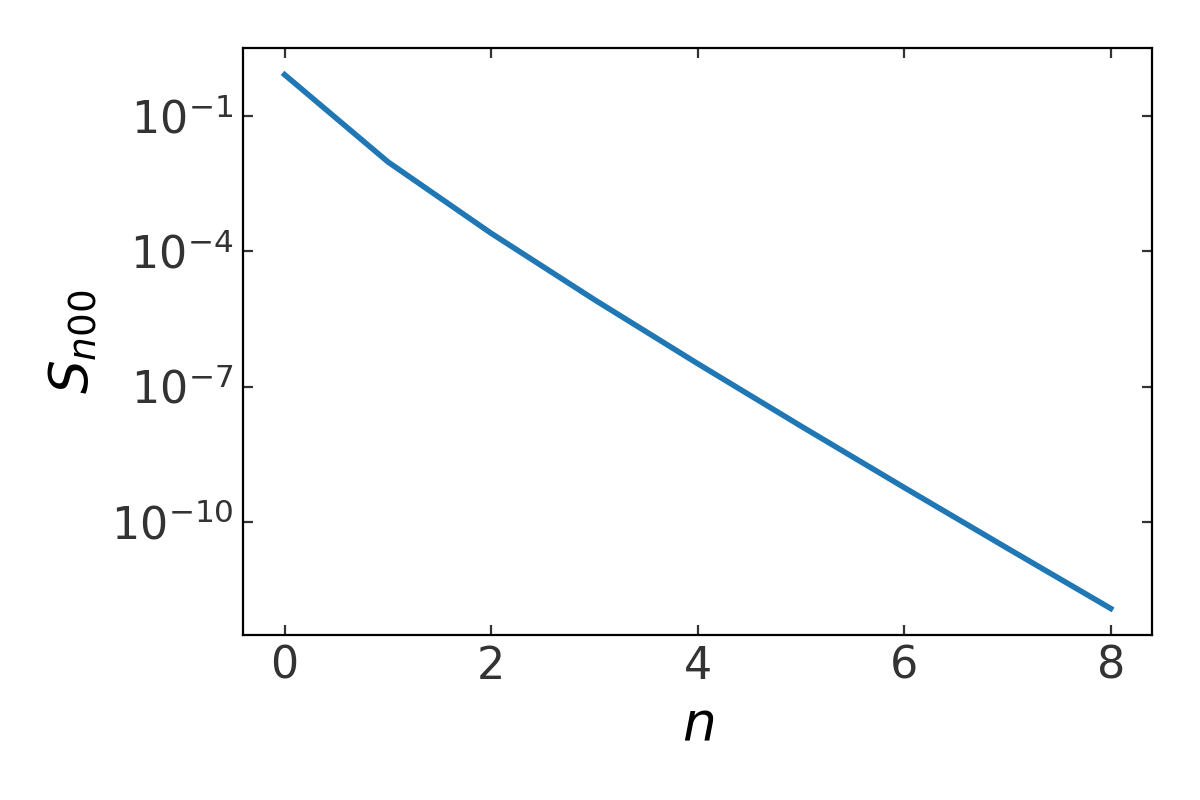
Now that we have the coefficients in hand, we can visualize their magnitudes:
plt.figure(figsize=(6,4))
plt.semilogy(np.abs(S[:,0,0]), marker=None, lw=2)
plt.xlabel("$n$")
plt.ylabel("$S_{n00}$")
(Source code, png, pdf)

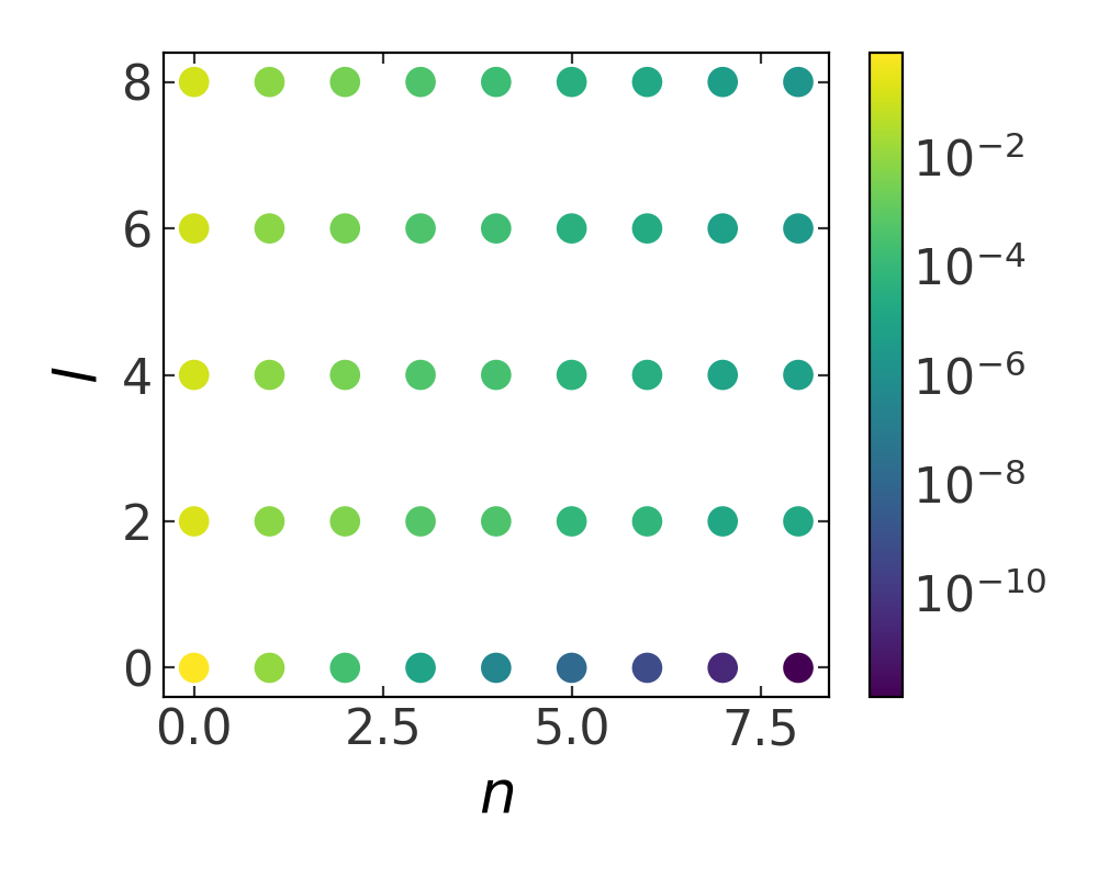
Because we ignored any \(m\) terms, the coefficients are computed in a 2D grid in \(n,l\): we can visualize their magnitude by coloring points on such a grid:
nl_grid = np.mgrid[0:lmax+1, 0:nmax+1]

plt.figure(figsize=(5,4))
plt.scatter(nl_grid[0].ravel(), nl_grid[1].ravel(),
            c=np.abs(S[:,:,0].ravel()), norm=mpl.colors.LogNorm(),
            cmap='viridis', s=80)
plt.xlabel('$n$')
plt.ylabel('$l$')
plt.colorbar()
(Source code, png, pdf)
Using SCFPotential to evaluate the density, potential, gradient#
In this example we’ll continue where the previous example left off: we now have computed expansion coefficients for a
given density function and we would like to evaluate the gradient of the
gravitational potential at various locations. We will use gala to integrate
an orbit in the expansion potential.
From the previous example, we have a set of cosine and sine coefficients (S
and T) for an SCF representation of a flattened (oblate) Hernquist density
profile. First, we’ll create an SCFPotential object using
these coefficients:
potential = scf.SCFPotential(Snlm=S, Tnlm=T, m=M, r_s=a) # M=a=1
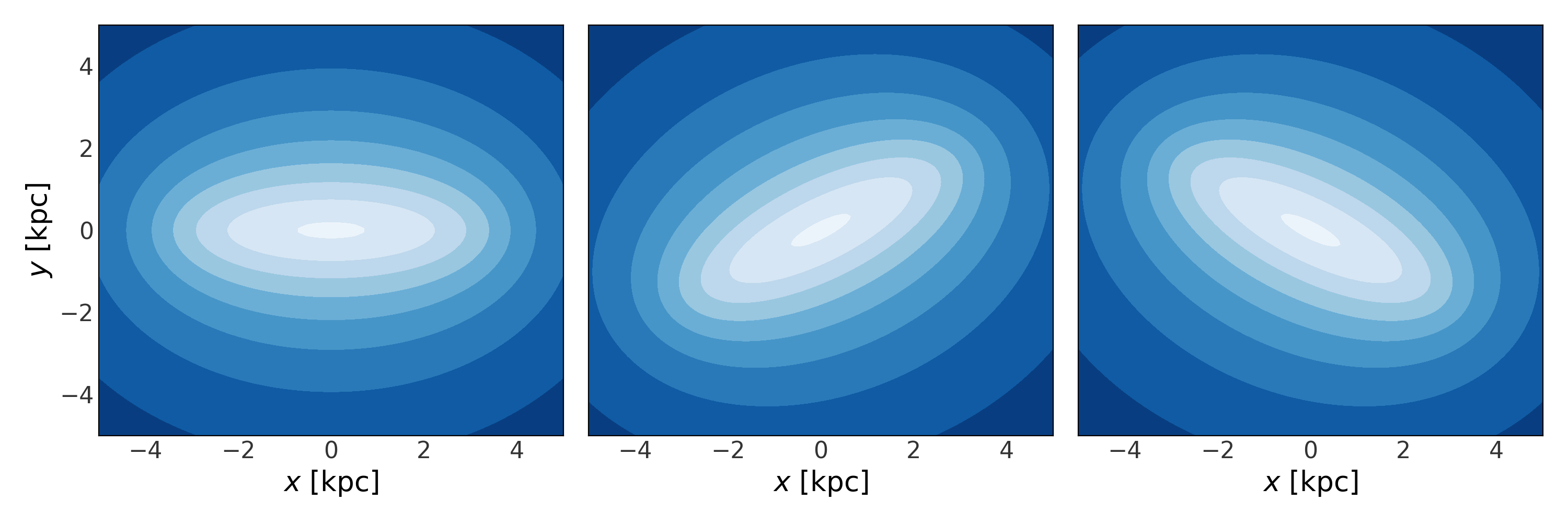
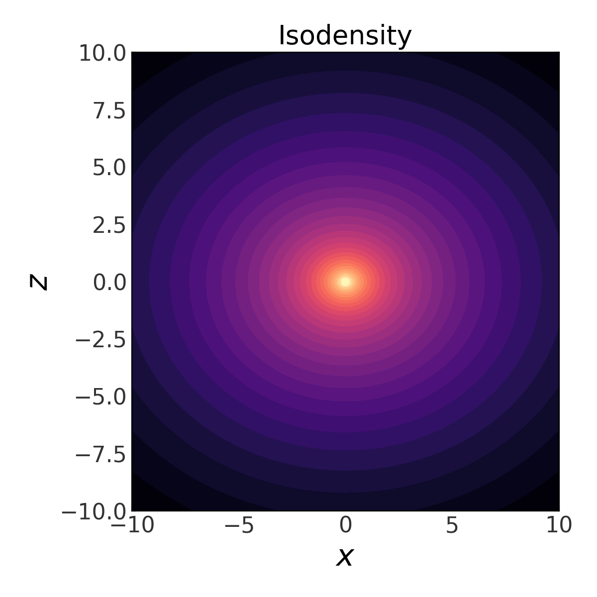
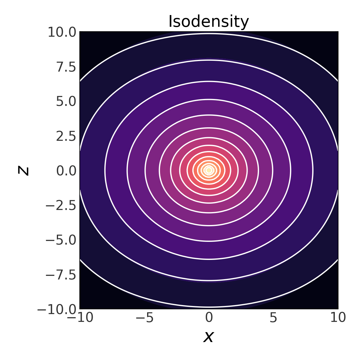
Let’s compare how our expansion density to the true density by recreating the above isodensity contour figure with SCF density contours overlaid:
x,z = np.meshgrid(np.linspace(-10., 10., 128),
                  np.linspace(-10., 10., 128))
y = np.zeros_like(x)
true_dens = flattened_hernquist_density(x, y, z, M, a, q)

# we need an array of positions with shape (3,n_samples) for SCFPotential
xyz = np.vstack((x.ravel(),y.ravel(),z.ravel()))
scf_dens = potential.density(xyz).value

# log-spaced contour levels
levels = np.logspace(np.log10(true_dens.min()), np.log10(true_dens.max()), 16)

plt.figure(figsize=(6,6))

plt.contourf(x, z, true_dens, cmap='magma',
             levels=levels, locator=ticker.LogLocator())
plt.contour(x, z, scf_dens.reshape(x.shape), colors='w',
            levels=levels, locator=ticker.LogLocator())

plt.title("Isodensity")
plt.xlabel("$x$", fontsize=22)
plt.ylabel("$z$", fontsize=22)
(Source code, png, pdf)

By eye, the SCF representation looks pretty good. Let’s now create a plot of
equipotential contours using the SCFPotential instance:
scf_pot = np.abs(potential.energy(xyz))
scf_pot = scf_pot.value # get numerical value from `~astropy.units.Quantity`

# log-spaced contour levels
levels = np.logspace(np.log10(scf_pot.min()), np.log10(scf_pot.max()), 16)

plt.figure(figsize=(6,6))

plt.contour(x, z, scf_pot.reshape(x.shape), cmap='inferno_r',
            levels=levels, locator=ticker.LogLocator())

plt.title("Equipotential")
plt.xlabel("$x$", fontsize=22)
plt.ylabel("$z$", fontsize=22)
(Source code, png, pdf)
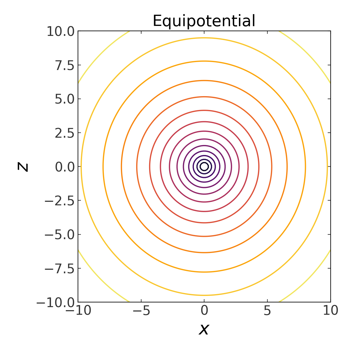
(the above is actually provided as a convenience method of any
PotentialBase subclass – see
plot_contours).
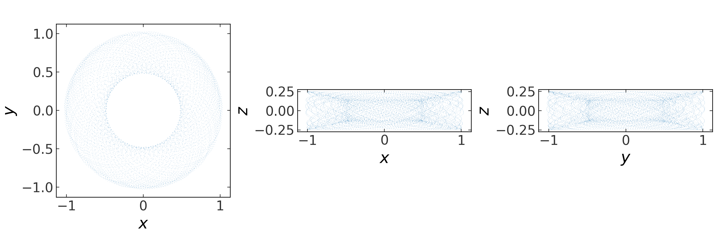
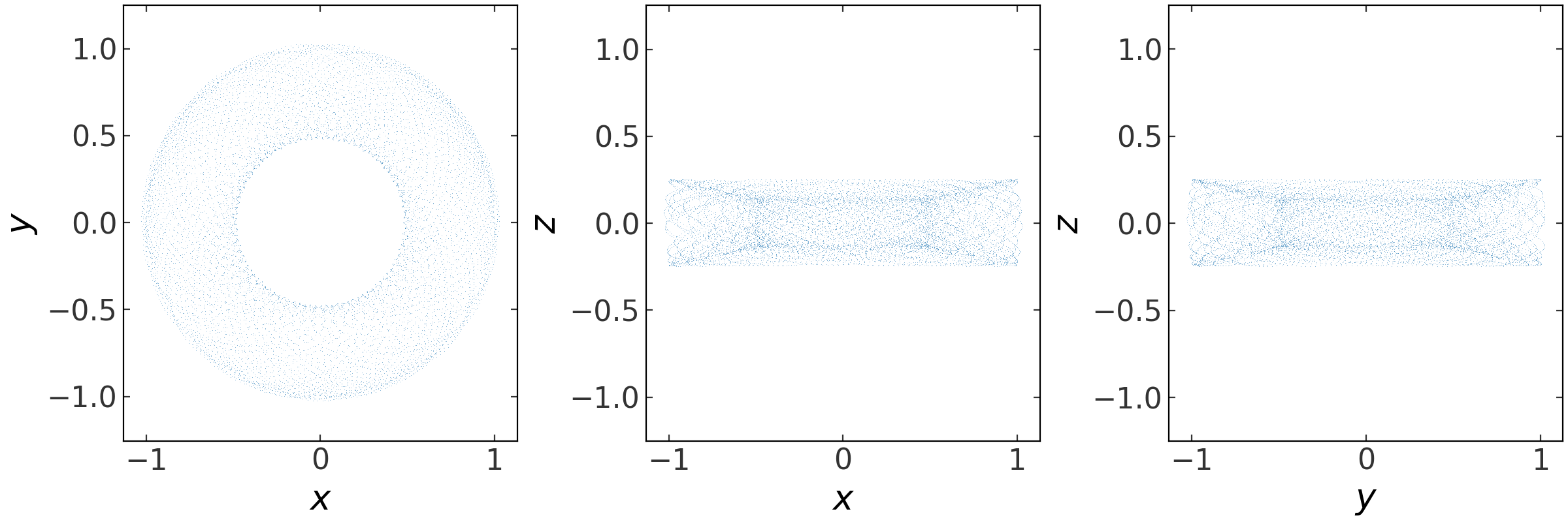
Now let’s integrate an orbit in this potential. We’ll use the orbit integration
framework from gala.integrate and the convenience method
integrate_orbit to do this:
import gala.dynamics as gd

# when using dimensionless units, we don't need to specify units for the
# initial conditions
w0 = gd.PhaseSpacePosition(pos=[1.,0,0.25],
                           vel=[0.,0.3,0.])

# by default this uses Leapfrog integration
orbit = potential.integrate_orbit(w0, dt=0.1, n_steps=10000)

fig = orbit_l.plot(marker=',', linestyle='none', alpha=0.5)
(Source code, png, pdf)