Orbit and phase-space position objects in more detail#
For the examples below the following imports have already been executed:
>>> import astropy.units as u
>>> import numpy as np
>>> import gala.potential as gp
>>> import gala.dynamics as gd
>>> from astropy.coordinates import (CylindricalRepresentation,
...                                  CylindricalDifferential)
>>> from gala.units import galactic
>>> np.random.seed(42)
We will also set the default Astropy Galactocentric frame parameters to the values adopted in Astropy v4.0:
>>> import astropy.coordinates as coord
>>> _ = coord.galactocentric_frame_defaults.set('v4.0')
Introduction#
The astropy.units subpackage is excellent for working with numbers and
associated units, but dynamical quantities often contain many quantities with
mixed units. An example is a position in phase-space, which may contain some
quantities with length units and some quantities with velocity or momentum
units. The PhaseSpacePosition and Orbit classes are designed to work with these data
structures and provide a consistent API for visualizing and computing further
dynamical quantities. Click these shortcuts to jump to a section below, or start
reading below:
Phase-space Positions#
The PhaseSpacePosition class provides an interface for representing full phase-space
positions–coordinate positions and momenta (velocities). This class is useful
as a container for initial conditions and for transforming phase-space positions
to new coordinate representations or reference frames.
The easiest way to create a PhaseSpacePosition object is to pass in a pair of
Quantity objects that represent the Cartesian position and
velocity vectors:
>>> gd.PhaseSpacePosition(pos=[4., 8., 15.] * u.kpc,
...                       vel=[-150., 50., 15.] * u.km/u.s)
<PhaseSpacePosition cartesian, dim=3, shape=()>
By default, passing in Quantity’s are interpreted as Cartesian
coordinates and velocities. This works with arrays of positions and velocities
as well:
>>> x = np.arange(24).reshape(3, 8)
>>> v = np.arange(24).reshape(3, 8)
>>> w = gd.PhaseSpacePosition(pos=x * u.kpc,
...                           vel=v * u.km/u.s)
>>> w
<PhaseSpacePosition cartesian, dim=3, shape=(8,)>
This is interpreted as 8, 6-dimensional phase-space positions.
The class internally stores the positions and velocities as
BaseRepresentation and
BaseDifferential subclasses; in this case,
CartesianRepresentation and
CartesianDifferential:
>>> w.pos
<CartesianRepresentation (x, y, z) in kpc
    [(0.,  8., 16.), (1.,  9., 17.), (2., 10., 18.), (3., 11., 19.),
     (4., 12., 20.), (5., 13., 21.), (6., 14., 22.), (7., 15., 23.)]>
>>> w.vel
<CartesianDifferential (d_x, d_y, d_z) in km / s
    [(0.,  8., 16.), (1.,  9., 17.), (2., 10., 18.), (3., 11., 19.),
     (4., 12., 20.), (5., 13., 21.), (6., 14., 22.), (7., 15., 23.)]>
All of the components of these classes are mapped to attributes of the
phase-space position class for convenience, but with more user-friendly names.
These mappings are defined in the class definition of
PhaseSpacePosition. For example, to access the x component
of the position and the v_x component of the velocity:
>>> w.x
<Quantity [0.,1.,2.,3.,4.,5.,6.,7.] kpc>
>>> w.v_x
<Quantity [0.,1.,2.,3.,4.,5.,6.,7.] km / s>
The default representation is Cartesian, but the class can also be instantiated
with representation objects instead of Quantity’s – this is
useful for creating PhaseSpacePosition or Orbit instances from non-Cartesian
representations of the position and velocity:
>>> pos = CylindricalRepresentation(rho=np.linspace(1., 4, 4) * u.kpc,
...                                 phi=np.linspace(0, np.pi, 4) * u.rad,
...                                 z=np.linspace(-1, 1., 4) * u.kpc)
>>> vel = CylindricalDifferential(d_rho=np.linspace(100, 150, 4) * u.km/u.s,
...                               d_phi=np.linspace(-1, 1, 4) * u.rad/u.Myr,
...                               d_z=np.linspace(-15, 15., 4) * u.km/u.s)
>>> w = gd.PhaseSpacePosition(pos=pos, vel=vel)
>>> w
<PhaseSpacePosition cylindrical, dim=3, shape=(4,)>
>>> w.rho
<Quantity [1., 2., 3., 4.] kpc>
We can easily transform the full phase-space vector to new representations or
coordinate frames. These transformations use the astropy.coordinates
representations framework:
>>> cart = w.represent_as('cartesian')
>>> cart.x
<Quantity [ 1. ,  1. , -1.5, -4. ] kpc>
>>> sph = w.represent_as('spherical')
>>> sph.distance
<Distance [1.41421356, 2.02758751, 3.01846171, 4.12310563] kpc>
There is also support for transforming the positions and velocities (assumed to
be in a Galactocentric frame) to any of the other
coordinate frames. For example, to transform to
Galactic coordinates:
>>> from astropy.coordinates import Galactic
>>> gal_c = w.to_coord_frame(Galactic())
>>> gal_c
<Galactic Coordinate: (l, b, distance) in (deg, deg, kpc)
    [(4.40971301e-05, -6.23850462, 9.17891228),
    (1.07501936e+01, -2.04017409, 9.29170644),
    (2.14246214e+01,  2.65220588, 7.12026744),
    (7.35169893e-05, 13.50991169, 4.23668468)]
(pm_l_cosb, pm_b, radial_velocity) in (mas / yr, mas / yr, km / s)
    [( -28.11596908, -0.297625  ,    89.093095  ),
    ( -13.077309  ,  0.15891073,   511.60269726),
    (  -7.04751509,  1.33976418, -1087.52574084),
    (-206.97042166,  2.22471526,  -156.82064814)]>
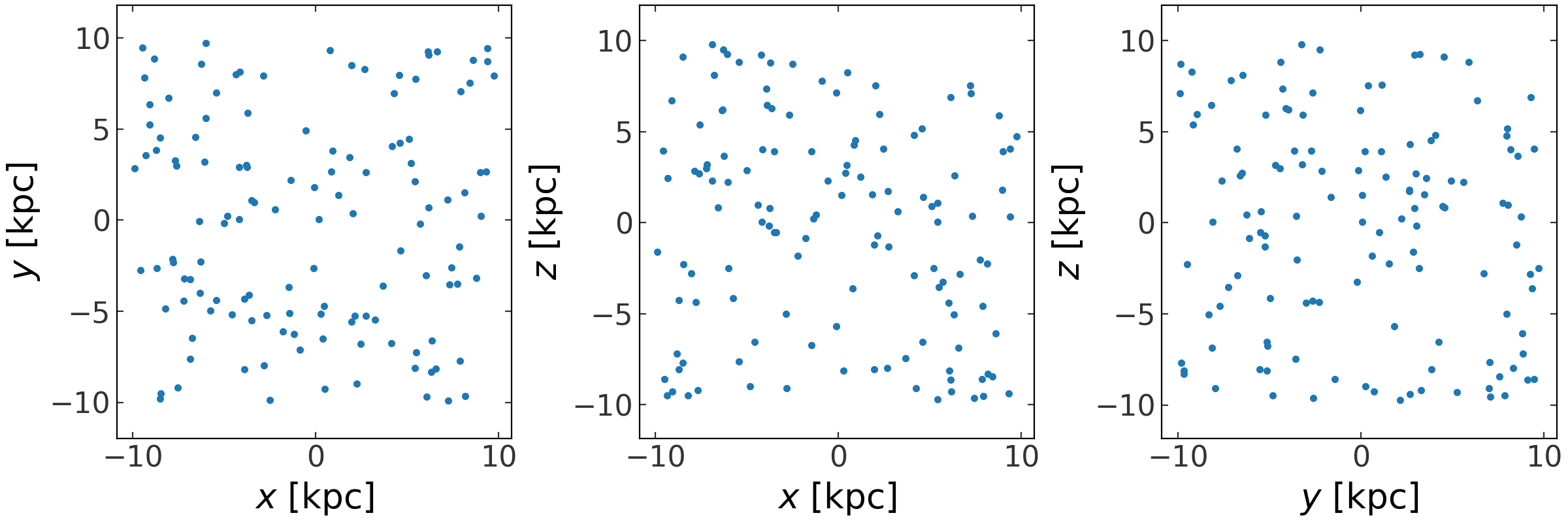
We can easily plot projections of the phase-space positions using the
plot method:
>>> np.random.seed(42)
>>> x = np.random.uniform(-10, 10, size=(3,128))
>>> v = np.random.uniform(-200, 200, size=(3,128))
>>> w = gd.PhaseSpacePosition(pos=x * u.kpc,
...                           vel=v * u.km/u.s)
>>> fig = w.plot()
(Source code, png, pdf)
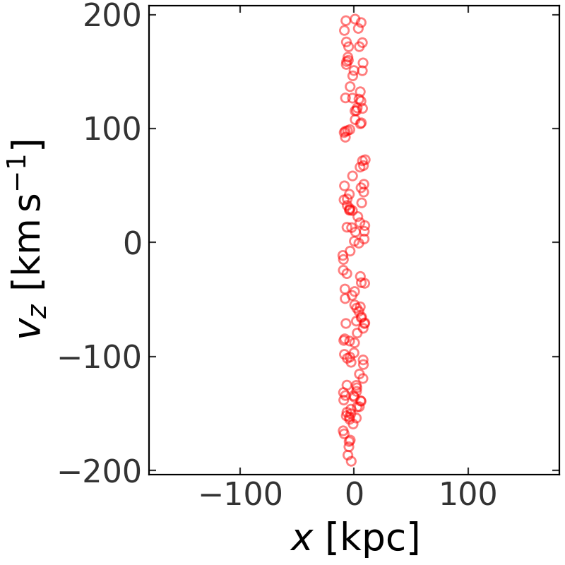
This is a thin wrapper around the plot_projections
function and any keyword arguments are passed through to that function:
>>> fig = w.plot(components=['x', 'v_z'], color='r',
...              facecolor='none', marker='o', s=20, alpha=0.5)
(Source code, png, pdf)
Orbits#
The Orbit class inherits much of the functionality from PhaseSpacePosition (described above)
and adds some additional features that are useful for time-series orbits.
An Orbit instance is initialized like the PhaseSpacePosition–with arrays of positions and
velocities– but usually also requires specifying a time array as well. Also,
the extra axes in these arrays hold special meaning for the Orbit class. The
position and velocity arrays passed to PhaseSpacePosition can have arbitrary numbers of
dimensions as long as the 0th axis specifies the dimensionality. For the Orbit
class, the 0th axis remains the axis of dimensionality, but the 1st axis now is
always assumed to be the time axis. For example, an input position with shape
(2,128) to a PhaseSpacePosition represents 128 independent 2D positions, but to a Orbit
it represents a single orbit’s positions at 128 times:
>>> t = np.linspace(0, 100, 128) * u.Myr
>>> Om = 1E-1 * u.rad / u.Myr
>>> pos = np.vstack((5*np.cos(Om*t), np.sin(Om*t))).value * u.kpc
>>> vel = np.vstack((-5*np.sin(Om*t), np.cos(Om*t))).value * u.kpc/u.Myr
>>> orbit = gd.Orbit(pos=pos, vel=vel)
>>> orbit
<Orbit ndcartesian, dim=2, shape=(128,)>
To create a single object that contains multiple orbits, the input position
object should have 3 axes. The last axis (axis=2) specifies the number of
orbits. So, an input position with shape (2,128,16) would represent 16, 2D
orbits, each with the same 128 times:
>>> t = np.linspace(0, 100, 128) * u.Myr
>>> Om = np.random.uniform(size=16) * u.rad / u.Myr
>>> angle = Om[None] * t[:, None]
>>> pos = np.stack((5*np.cos(angle), np.sin(angle))).value * u.kpc
>>> vel = np.stack((-5*np.sin(angle), np.cos(angle))).value * u.kpc/u.Myr
>>> orbit = gd.Orbit(pos=pos, vel=vel)
>>> orbit
<Orbit ndcartesian, dim=2, shape=(128, 16)>
To make full use of the orbit functionality, you must also pass in an array with
the time values and an instance of a PotentialBase
subclass that represents the potential that the orbit was integrated in:
>>> pot = gp.PlummerPotential(m=1E10, b=1., units=galactic)
>>> orbit = gd.Orbit(pos=pos*u.kpc, vel=vel*u.km/u.s,
...                  t=t*u.Myr, potential=pot)
(note, in this case pos and vel were not generated from integrating
an orbit in the potential pot!). However, most of the time you won’t need to
create Orbit objects from scratch! They are returned from any of the numerical
integration routines provided in gala. For example, they are returned by the
integrate_orbit method of potential
objects and will automatically contain the time array and potential
object. For example:
>>> pot = gp.PlummerPotential(m=1E10 * u.Msun, b=1. * u.kpc, units=galactic)
>>> w0 = gd.PhaseSpacePosition(pos=[10.,0,0] * u.kpc,
...                            vel=[0.,75,0] * u.km/u.s)
>>> orbit = gp.Hamiltonian(pot).integrate_orbit(w0, dt=1., n_steps=5000)
>>> orbit
<Orbit cartesian, dim=3, shape=(5001,)>
>>> orbit.t
<Quantity [0.000e+00, 1.000e+00, 2.000e+00, ..., 4.998e+03, 4.999e+03,
           5.000e+03] Myr>
>>> orbit.potential
<PlummerPotential: m=1.00e+10, b=1.00 (kpc,Myr,solMass,rad)>
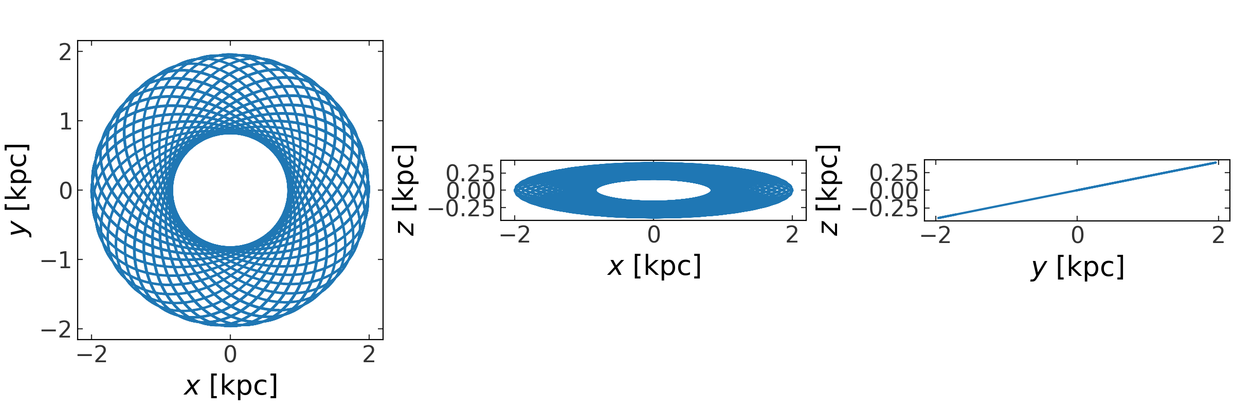
Just like for PhaseSpacePosition, we can quickly visualize an orbit using the
plot method:
>>> fig = orbit.plot()
(Source code, png, pdf)
Again, this is a thin wrapper around the plot_projections
function and any keyword arguments are passed through to that function:
>>> fig = orbit.plot(linewidth=4., alpha=0.5, color='r')
(Source code, png, pdf)
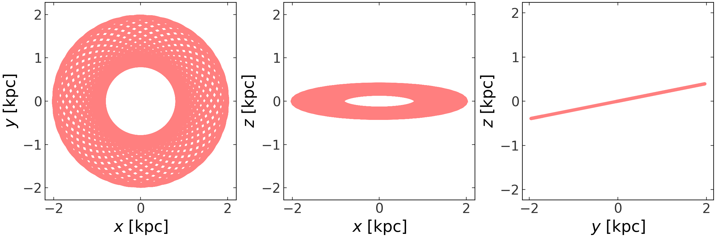

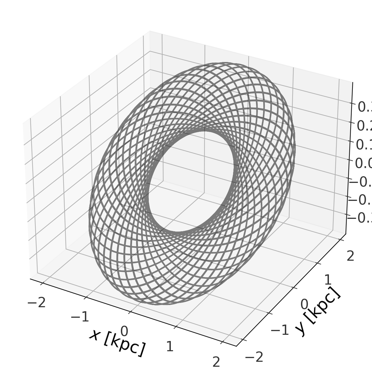
Alternatively, for three-dimensional orbits, we can visualize the orbit using
the 3D projection capabilities in matplotlib:
>>> fig = orbit.plot_3d(alpha=0.5, color='k')
(Source code, png, pdf)
We can also quickly create an animation of the progression of an orbit using the
animate method, which animated projections of the orbit:
>>> fig, anim = orbit[:1000].animate(stride=10)
The animate method acts like plot, in that it works for
any coordinate representation (Cartesian, cylindrical, etc.) and supports only
animating subsets of the phase-space components. For example, to make an
animation of an orbit in cylindrical coordinates, showing the orbit proress in
the R,z meridional plane:
>>> fig, anim = orbit[:1000].cylindrical.animate(components=['rho', 'z'],
...                                              stride=10)
We can also quickly compute quantities like the angular momentum, and estimates for the pericenter, apocenter, eccentricity of the orbit. Estimates for the latter few get better with smaller timesteps:
>>> orbit = gp.Hamiltonian(pot).integrate_orbit(w0, dt=0.1, n_steps=100000)
>>> np.mean(orbit.angular_momentum(), axis=1)
<Quantity [0.        ,0.        ,0.76703412] kpc2 / Myr>
>>> orbit.eccentricity()
<Quantity 0.31951765618193967>
>>> orbit.pericenter()
<Quantity 10.00000005952518 kpc>
>>> orbit.apocenter()
<Quantity 19.390916871970223 kpc>
More information#
Internally, both of the above classes rely on the Astropy representation
transformation framework (i.e. the subclasses of
BaseRepresentation and
BaseDifferential). However, at present these classes only
support 3D positions and differentials (velocities). The PhaseSpacePosition and Orbit classes
both support arbitrary numbers of dimensions and, when relevant, rely on custom
subclasses of the representation classes to handle such cases. See the
N-dimensional representation classes page for more information about these classes.