N-body (gala.dynamics.nbody)#
Introduction#
With the Hamiltonian and potential classes
(potential), Gala contains functionality for integrating test particle
orbits in background gravitational fields. To supplement this, Gala also now
contains some limited functionality for performing N-body orbit integrations
through direct N-body force calculations between particles. With the
gala.dynamics.nbody subpackage, gravitational fields (i.e., any potential
class from gala.potential) can be sourced by particles that interact, and
optionally feel a background/external potential. To use this functionality, the
core class is DirectNBody. Below, we’ll go through a few
examples of using this class to perform orbit integrations
For the examples below the following imports have already been executed:
>>> import astropy.units as u
>>> import numpy as np
>>> import gala.potential as gp
>>> import gala.dynamics as gd
>>> from gala.dynamics.nbody import DirectNBody
>>> from gala.units import galactic, UnitSystem
Getting started#
The DirectNBody, at minimum, must be instantiated with a
set of particle orbital initial conditions along with a specification of the
gravitational fields sourced by each particle — that is, the number of initial
conditions must match the input list of gravitational potential objects that
specify the particle mass distributions. Other optional arguments to
DirectNBody allow you to set the unit system (i.e., to
improve numerical precision when time-stepping the orbit integration), or to
specify a background gravitational potential. Let’s now go through a few
examples of using this class in practice.
Example: Mixed test particle and massive particle orbit integration#
Like with Hamiltonian orbit integration, orbital
initial conditions are passed in to DirectNBody by
passing in a single PhaseSpacePosition object. Let’s create two
initial conditions by specifying the position and velocity of two particles,
then combine them into a single PhaseSpacePosition object:
>>> w0_1 = gd.PhaseSpacePosition(pos=[0, 0, 0] * u.pc,
...                              vel=[0, 1.5, 0] * u.km/u.s)
>>> w0_2 = gd.PhaseSpacePosition(pos=w0_1.xyz + [100., 0, 0] * u.pc,
...                              vel=w0_1.v_xyz + [0, 5, 0] * u.km/u.s)
>>> w0 = gd.combine((w0_1, w0_2))
>>> w0.shape
(2,)
We’ll then treat particle 1 as a massive object by sourcing a
HernquistPotential at the location of the particle,
and particle 2 as a test particle: To treat some particles as test particles,
you can pass None or a NullPotential instance
for the corresponding particle potential:
>>> pot1 = gp.HernquistPotential(m=1e7*u.Msun, c=0.5*u.kpc, units=galactic)
>>> particle_pot = [pot1, None]
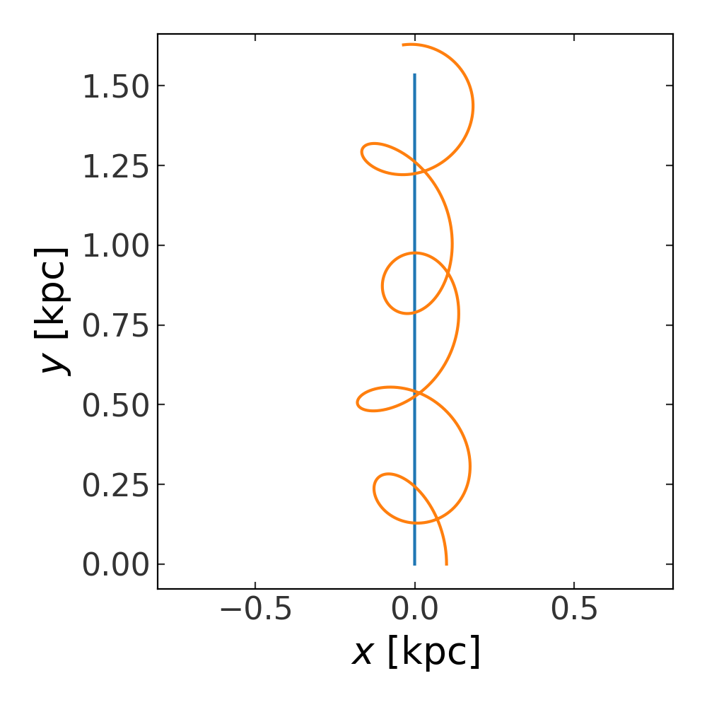
Let’s now create an N-body instance and try integrating the orbits of the two particles. Here, there is no external potential, so particle 1 (the massive particle) will move off in a straight line. We’ve created the initial conditions for particle 2 so that it will remain bound to the potential sourced by particle 1, and so will orbit it as it moves. Let’s create the object and integrate the orbits:
>>> nbody = DirectNBody(w0, particle_pot)
>>> orbits = nbody.integrate_orbit(dt=1e-2*u.Myr, t1=0, t2=1*u.Gyr)
>>> fig, ax = plt.subplots(1, 1, figsize=(5, 5))
>>> _ = orbits[:, 0].plot(['x', 'y'], axes=[ax])
>>> _ = orbits[:, 1].plot(['x', 'y'], axes=[ax])
(Source code, png, pdf)

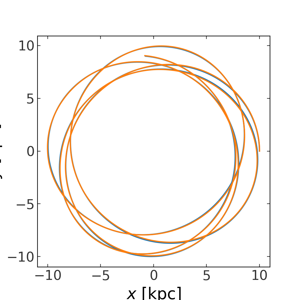
Example: N-body integration with a background potential#
With DirectNBody, we can also specify a background or
external potential to integrate all orbits in. To do this, you can optionally
pass in an external potential as a potential object to
DirectNBody. Here, as an example, we’ll repeat a similar
integration as above, but (1) add a positional offset of the initial conditions
from the origin, and (2) specify an external potential using the
MilkyWayPotential class as an external potential:
>>> external_pot = gp.MilkyWayPotential(version="latest")
>>> w0_1 = gd.PhaseSpacePosition(pos=[10, 0, 0] * u.kpc,
...                              vel=[0, 200, 0] * u.km/u.s)
>>> w0_2 = gd.PhaseSpacePosition(pos=w0_1.xyz + [10., 0, 0] * u.pc,
...                              vel=w0_1.v_xyz + [0, 5, 0] * u.km/u.s)
>>> w0 = gd.combine((w0_1, w0_2))
>>> pot1 = gp.HernquistPotential(m=1e7*u.Msun, c=0.5*u.kpc, units=galactic)
>>> particle_pot = [pot1, None]
>>> nbody = DirectNBody(w0, particle_pot, external_potential=external_pot)
>>> orbits = nbody.integrate_orbit(dt=1e-2*u.Myr, t1=0, t2=1*u.Gyr)
>>> fig, ax = plt.subplots(1, 1, figsize=(5, 5))
>>> _ = orbits[:, 0].plot(['x', 'y'], axes=[ax])
>>> _ = orbits[:, 1].plot(['x', 'y'], axes=[ax])
(Source code, png, pdf)

In this case, the orbits are so similar that it is hard to tell whether the test particle is actually bound to the secondary mass. Let’s instead now plot the position in the x-y plane of particle 2 relative to particle 1. This will look strange because we have not transformed to the frame of particle 1, but it should give us a sense of whether particle 2 is bound or unbound to this mass:
>>> dxyz = orbits[:, 0].xyz - orbits[:, 1].xyz
>>> fig, ax = plt.subplots(1, 1, figsize=(5, 5))
>>> ax.plot(dxyz[0], dxyz[1])
(Source code, png, pdf)
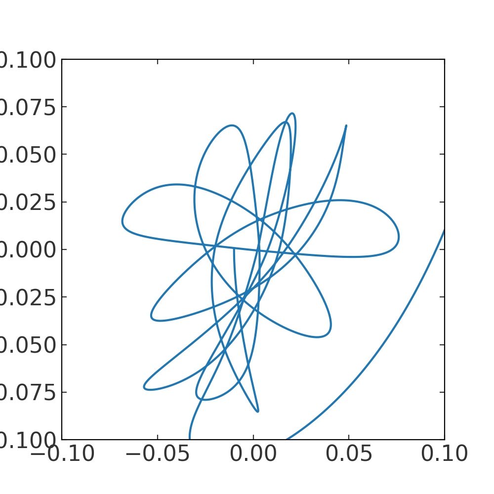
From this, it looks like particle 2 is indeed still bound to particle 1 as they both orbit within the external potential.
gala.dynamics.nbody Package#
Classes#
|
Perform orbit integration using direct N-body forces between particles, optionally in an external background potential. |