Defining your own potential class#
Introduction#
There are two ways to define a new potential class: with pure-Python, or with C and Cython. The advantage to writing a new class in Cython is that the computations can execute with C-like speeds, however only certain integrators support using this functionality (Leapfrog and DOP853) and it is a bit more complicated to set up the code to build the C+Cython code properly. If you are not familiar with Cython, you probably want to stick to a pure Python class for initial testing. If there is a potential class that you think should be included as a built-in Cython potential, feel free to suggest the new addition as a GitHub issue!
For the examples below the following imports have already been executed:
>>> import numpy as np
>>> import gala.potential as gp
>>> import gala.dynamics as gd
Implementing a new potential with Python#
New Python potentials are implemented by subclassing
PotentialBase and defining functions that
compute (at minimum) the energy and gradient of the potential. We will work
through an example below for adding the Henon-Heiles potential.
The expression for the potential is:
With this parametrization, there is only one free parameter (A), and the
potential is two-dimensional.
At minimum, the subclass must implement the following methods:
__init__()_energy()_gradient()
The _energy() method should compute the potential energy at a given position
and time. The _gradient() method should compute the gradient of the
potential. Both of these methods must accept two arguments: a position, and a
time. These internal methods are then called by the
PotentialBase superclass methods
energy() and
gradient(). The superclass methods
convert the input position to an array in the unit system of the potential for
fast evaluation. The input to these superclass methods can be
Quantity objects,
PhaseSpacePosition objects, or ndarray.
Because this potential has a parameter, the __init__ method must accept
a parameter argument and store this in the parameters dictionary attribute
(a required attribute of any subclass). Let’s write it out, then work through
what each piece means in detail:
>>> class CustomHenonHeilesPotential(gp.PotentialBase):
...     A = gp.PotentialParameter("A")
...     ndim = 2
...
...     def _energy(self, xy, t):
...         A = self.parameters['A'].value
...         x,y = xy.T
...         return 0.5*(x**2 + y**2) + A*(x**2*y - y**3/3)
...
...     def _gradient(self, xy, t):
...         A = self.parameters['A'].value
...         x,y = xy.T
...
...         grad = np.zeros_like(xy)
...         grad[:,0] = x + 2*A*x*y
...         grad[:,1] = y + A*(x**2 - y**2)
...         return grad
The internal energy and gradient methods compute the numerical value and
gradient of the potential. The __init__ method must take a single argument,
A, and store this to a parameter dictionary. The expected shape of the
position array (xy) passed to the internal _energy() and _gradient()
methods is always 2-dimensional with shape (n_points, n_dim) where
n_points >= 1 and n_dim must match the dimensionality of the potential
specified in the initializer. Note that this is different from the shape
expected when calling the public methods energy() and gradient()!
Let’s now create an instance of the class and see how it works. For now, let’s
pass in None for the unit system to designate that we’ll work with
dimensionless quantities:
>>> pot = CustomHenonHeilesPotential(A=1., units=None)
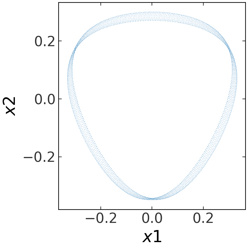
That’s it! We now have a potential object with all of the same functionality as the built-in potential classes. For example, we can integrate an orbit in this potential (but note that this potential is two-dimensional, so we only have to specify four coordinate values):
>>> w0 = gd.PhaseSpacePosition(pos=[0., 0.3],
...                            vel=[0.38, 0.])
>>> orbit = gp.Hamiltonian(pot).integrate_orbit(w0, dt=0.05, n_steps=10000)
>>> fig = orbit.plot(marker=',', linestyle='none', alpha=0.5)
(Source code, png, pdf)
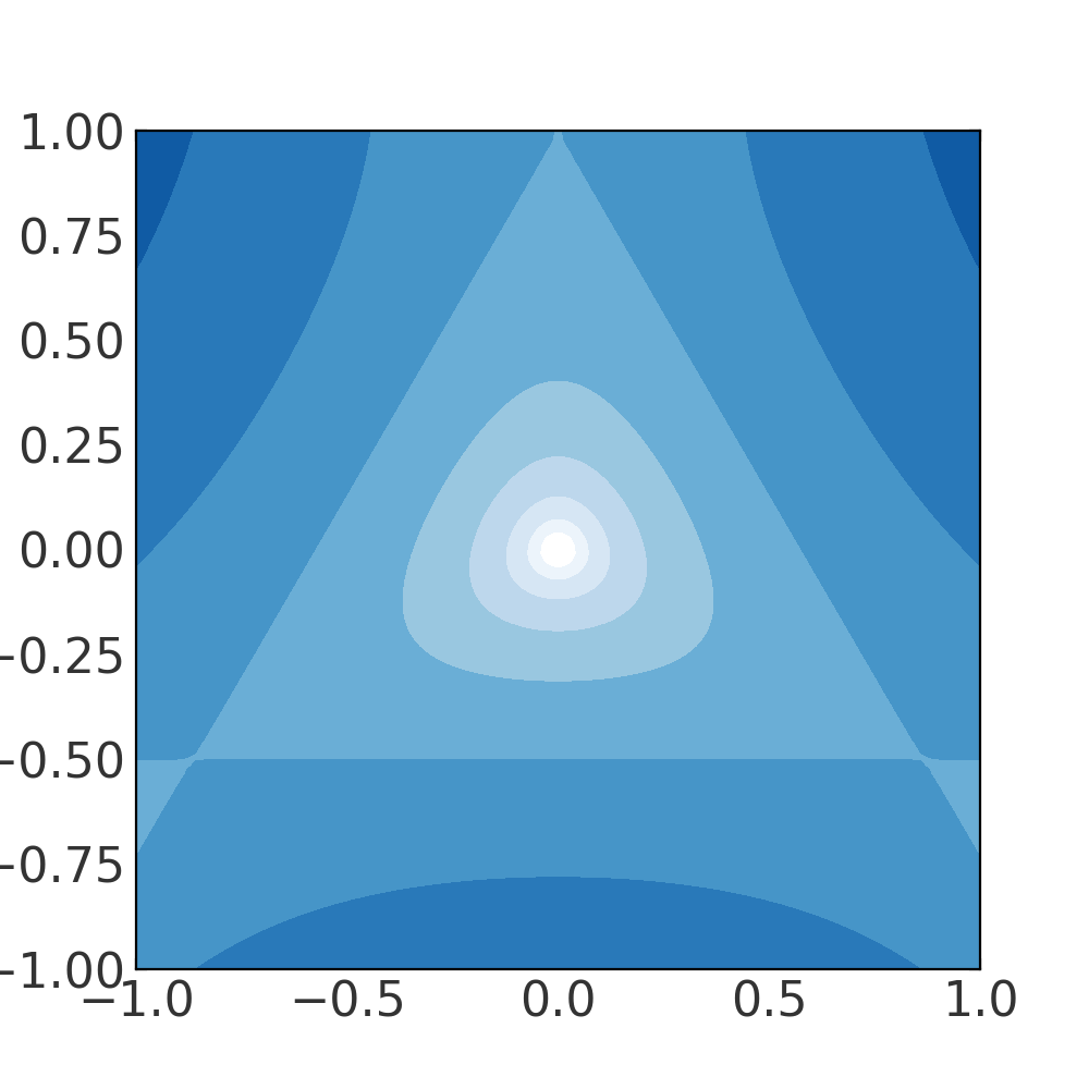
We could also, for example, create a contour plot of equipotentials:
>>> grid = np.linspace(-1., 1., 100)
>>> from matplotlib import colors
>>> import matplotlib.pyplot as plt
>>> fig, ax = plt.subplots(1, 1, figsize=(5,5))
>>> fig = pot.plot_contours(grid=(grid, grid),
...                         levels=np.logspace(-3, 1, 10),
...                         norm=colors.LogNorm(),
...                         cmap='Blues', ax=ax)
(Source code, png, pdf)
Adding a custom potential with Cython#
Adding a new Cython potential class is a little more involved as it requires writing C-code and setting it up properly to compile when the code is built. For this example, we’ll work through how to define a new C-implemented potential class representation of a Keplerian (point-mass) potential. Because this example requires using Cython to build code, we provide a separate demo GitHub repository with an implementation of this potential with a demonstration of a build system that successfully sets up the code.
New Cython potentials are implemented by subclassing
CPotentialBase, subclassing
CPotentialWrapper, and defining C functions
that compute (at minimum) the energy and gradient of the potential. This
requires creating (at minimum) a Cython file (.pyx), a C header file (.h), and a
C source file (.c).